To track the experiments, manage the models, and deploy the models, MLflow is a platform that manages the entire machine learning lifecycle. Machine learning models can be saved in a standard format called MLflow Models with the help of MLflow. Different flavors of MLflow Models can be saved, and each flavor is compatible with a particular set of downstream tools.
Saving a Model with MLflow
Use the mlflow.log_model() function to log a machine learning model in MLflow. These are the arguments that this function accepts:
- model: The model object to be saved.
- artifact_path: The path to the artifact where the model will be saved.
- flavor: The flavor of the model.
- registered_model_name: The model’s name is entered into the MLflow Model Registry.
Loading a Model with MLflow
- The mlflow.load_model() function
Benefits of Saving the Machine Learning Models with MLflow
- Standardized format: MLflow Models are standardized, easy to share with other tools.
- Version control: MLflow models can be easily updated through versioning.
- Model registry: MLflow provides a model registry for storage and management.
- Deployment: MLflow models can be quickly deployed to production.
Syntax of MLflow Model
To save a scikit-learn model as an MLflow model, for instance, use the following code:
Let’s implement the methods to save the machine learning models with MLflow for Medical Store Inventory System.
Scenario:
Let’s create a machine learning data model based on a medical store inventory system scenario that is used to predict the demand for different medical products in the year 2020. The aim is to optimize the inventory system by indicating the quantity of each product that is likely to be sold soon to help the store avoid stock-outs and excess inventory of different products.
Install the Prerequisite Libraries:
Install MLflow if it is not yet installed using the pip command:
![]()
Part 1: Data Generation
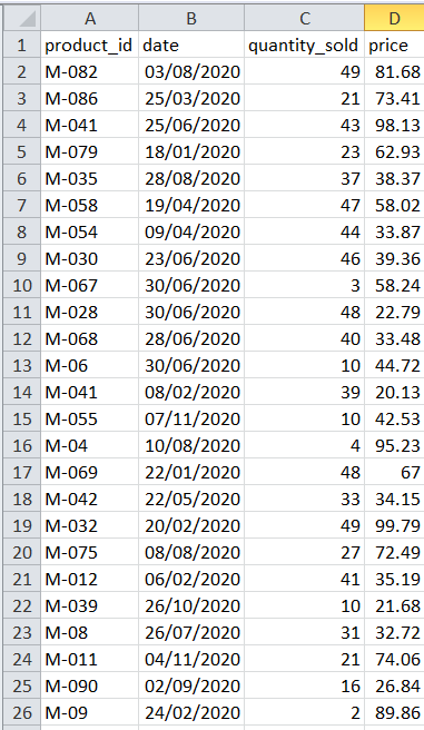
To generate a random medical store inventory data includes historical sales data for various medical products over time. The dataset consists of medicine items information like product ID, date of sale, quantity sold, and sale price. A machine learning model is created using this data to predict the demand for various drugs and medical supplies.
Code Snippet:
The code imports the Pandas, NumPy, random, and datetime libraries for data analysis, scientific computing, and date-time manipulation. In order to generate the sales data from 100 medical product IDs and item data, the code specifies the variables like sale_data_rows, product_ids, item_data, and start_date. The method creates random sales data by looping over the sale_data_rows and extending a new list for each item which contains the product ID, sale date, amount sold, and price.
Using the Pandas library, the code generates a sales_df dataframe with columns for product_id, date, quantity_sold, and sale price from an item_data list. Save it with the index option set to False in a CSV file.
import numpy
import random as rnd
from datetime import datetime as dt, timedelta as td
# Number of rows (sales records) to generate
sale_data_rows = 2000
# Generate List of medical product IDs
product_ids = [f'M-0{i}' for i in range(1, 100)]
# Generate random sales items data
item_data = []
begin_date = dt(2020, 1, 1)
for _ in range(sale_data_rows):
product_id = rnd.choice(product_ids)
product_sale_date = begin_date + td(days=rnd.randint(0, 365))
product_quantity_sold = rnd.randint(1, 50)
product_price = round(rnd.uniform(10, 100), 2)
item_data.append([product_id, product_sale_date, product_quantity_sold, product_price])
# Create a DataFrame from the generated data
name_columns = ['product_id', 'date', 'quantity_sold', 'price']
# create sales data frame using columns and item_date
sales_df = obj_pn.DataFrame(item_data, columns=name_columns)
# Save the DataFrame to medical_stores_sales CSV file
sales_df.to_csv('medical_stores_sales.csv', index=False)
# print success message
print("medical_stores_sales.csv generated successfully!")
![]()
Part 2: Data Processing and Set Tracking the URI
Preparing the data is a necessary step before training a machine learning model. The preparation of the data that has been collected is covered in this section. This includes handling the missing values, scalability of numerical features, encoding of categorical variables, and splitting the data into training and testing sets. The data must be correctly preprocessed to ensure that it can be used for model training and evaluation.
Code Explanation:
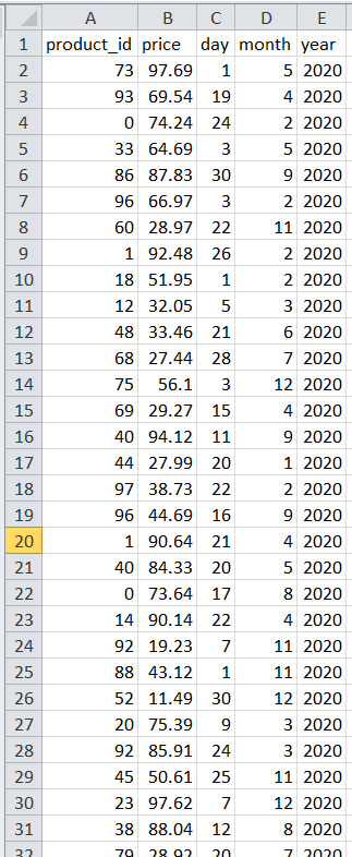
The necessary Python libraries are imported, and the “medical_stores_sales.csv” file contains the dataset of medications. The preprocessing function splits the data into features and targets, encrypts the product_id, and extracts the day, month, and year features. The data is divided into training and test sets, a Random Forest Regressor (RFR) model is initialized, trained, and evaluated, the metrics are logged, and the model is saved.
from sklearn.model_selection import train_test_split as tts
from sklearn.ensemble import RandomForestRegressor as RFR
from sklearn.metrics import mean_absolute_error, mean_squared_error
import mlflow
import mlflow.sklearn
from sklearn.preprocessing import LabelEncoder as LE
import os
os.environ["GIT_PYTHON_REFRESH"] = "quiet"
medicine_data = obj_pd.read_csv('medical_stores_sales.csv')
# Preprocess the data of pharmacy or medical store
# In this example, we will encode the 'product_id' column using LabelEncoder
id_le = LE()
medicine_data['product_id'] = id_le.fit_transform(medicine_data['product_id'])
# Extract day, month, and year features from the 'date' column
medicine_data['date'] = obj_pd.to_datetime(medicine_data['date'])
medicine_data['day'] = medicine_data['date'].dt.day
medicine_data['month'] = medicine_data['date'].dt.month
medicine_data['year'] = medicine_data['date'].dt.year
# Split the medicine data into features (F) and target (t)
F = medicine_data.drop(columns=['date', 'quantity_sold'])
t = medicine_data['quantity_sold']
F_training, F_testing, t_training, t_testing = tts(F, t, test_size=0.2, random_state=40)
mlflow.set_tracking_uri(‘http://127.0.0.1:5000’)
Part 3: Choose the Model
This part aims to select a model for a scenario that involves the management of an inventory in a medical supply store. Predicting each medical product’s anticipated future sales volume is the objective. We study the several regression techniques such as GBR (Gradient Boosting Regression), LR (Linear Regression), and Random Forest Regression (RFR). The chosen model needs to be able to forecast the numerical quantities which, in this case, is the number of the supplied medical supplies.
The code generates a supervised machine learning algorithm for regression tasks by importing the RandomForestRegressor class from the sklearn.ensemble package. It builds a forest of decision trees to produce the final predictions and averages them. The random_state option provides repeatability while the n_estimators parameter regulates the number of trees.
Code Snippet:
Part 4: Model Training and Evaluation
We then proceed to model training and evaluation once the optimal regression model has been selected. The use of the preprocessed data to train the chosen model is covered in this section.
Code Snippet with Explanation:
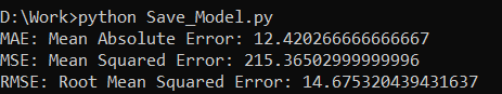
Before fitting the data and target values, RandomForestRegressor is accomplished on the training data. Using the predict() method, the code anticipates the test data. The code compares the predicted values by evaluating the model using the MAE, MSE, and RMSE metrics. Mean_squared_error() computes the differences in squared value, while root_mean_squared_error() computes the square. The mean_absolute_error() calculates the variations in terms of the absolute value. The importance of the three metrics are then printed by the code.
rfr_model.fit(F_training, t_training)
model_predictions = rfr_model.predict(F_testing)
# Evaluate the model
mae = mabse(t_testing, model_predictions)
mse = mserr(t_testing, model_predictions)
rmse = mserr(t_testing, model_predictions, squared=False)
print(f"MAE: Medicine Mean Absolute Error: {mae}")
print(f"MSE: Medicine Mean Squared Error: {mse}")
print(f"RMSE: Medicine Root Mean Squared Error: {rmse}")
Part 5: Save the ML Model with MLflow
In this final section, we look at how to train a machine learning model and how to store it using the Python MLflow module. An open-source platform called MLflow makes managing the full machine learning lifecycle easier. We will show how to log the model along with all the accompanying metadata such as the parameters and other pertinent tags. We can quickly replicate the model, share it with the team members, and deploy it to production for a real-time demand forecast in the medical store inventory management system by saving the model using MLflow.
Code Snippet:
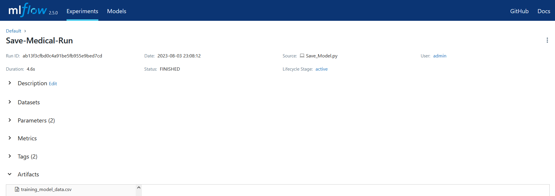
The code saves a machine learning model, parameters, and training data to MLflow using the “mlflow” library. Because of this, you may control the experiment, keep track of its progress, and replicate the results.
# Log the model and its parameters
mlflow.log_param("n_estimators", 150)
mlflow.log_param("random_state", 40)
# Log the model
mlflow.sklearn.save_model(rfr_model, "medical_store_prediction_model")
# Log additional metadata if needed
mlflow.set_tag("data_source", "medical_stores_sales.csv")
mlflow.set_tag("model_type", "RandomForestRegressor")
# Save the training data as an artifact
F_training.to_csv("training_model_data.csv", index=False)
mlflow.log_artifact("training_model_data.csv")
Part 6: Execute the Code

Conclusion
It is very simple to save, load, deploy, and track the machine learning models with the help of MLflow. It offers a uniform method of saving the models which facilitates sharing and deployment. To monitor and enhance the models, it also tracks the effectiveness of the data and the models that are created.