MLflow and TensorFlow Integration

The popular deep learning and machine learning framework, TensorFlow is developed by Google. To manage the machine learning’s whole lifecycle, MLflow is another open-source platform. It offers a range of tools for monitoring, controlling, and deploying the machine learning models. To monitor the development and testing of TensorFlow models, MLflow can be integrated with TensorFlow. For model monitoring, experiment management, and teamwork in machine learning projects, MLflow and TensorFlow integration can be helpful. Several advantages are offered by this connection, including:

Centralized tracking: The metrics, parameters, and artifacts related to a TensorFlow model are all tracked centrally by MLflow. This makes it simple to compare several models and to follow a model’s development over time.

Reproducibility: A TensorFlow model’s training and assessment can be duplicated using MLflow. This is crucial to ensuring that a model can be used in production and that its results can be replicated.

Deployment: MLflow can be used to deploy the TensorFlow models to production. This makes it easy to get the models into production and to track the performance of models in production.

To integrate MLflow with TensorFlow, you can use the “mlflow.tensorflow” module. This module provides a number of functions to log the metrics, parameters, and artifacts from the TensorFlow models.

Here are the steps to integrate MLflow with TensorFlow for model tracking:

Step 1: Install the Required Libraries

Make sure to have both MLflow and TensorFlow installed. To install MLflow, use the pip command that is given in the following:

pip install mlflow

To install TensorFlow, use the pip command:

pip install mlflow tensorflow

Step 2: Set Up an MLflow Tracking Server (Optional)

It totally depends upon the end-user requirements, either to install the local MLflow tracking server or the remote one. Use the command that is mentioned here to set up the local MLflow tracking server. With this command, the tracking server is started on the local machine, and it is accessible using port 5000 by default.

mlflow server

Step 3: Import the Libraries and Start an MLflow Run

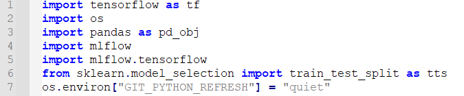
To use the TensorFlow framework in the code, the listed libraries are needed to build and run the code in Python.

Import MLflow
Import Mlflow.tensorflow
Import TensorFlow

Real World Scenario to Use the TensorFlow Framework:

Here, we envision a hypothetical medical research organization that works to create a machine-learning model for disease prediction using a patient data. Before accessing the actual patient data, the institute must provide a synthetic data to prototype and test their algorithms. A dataset with medical features and associated disease labels is to be created to simulate an actual scenario.

Step 4: Data Collection and Preparation

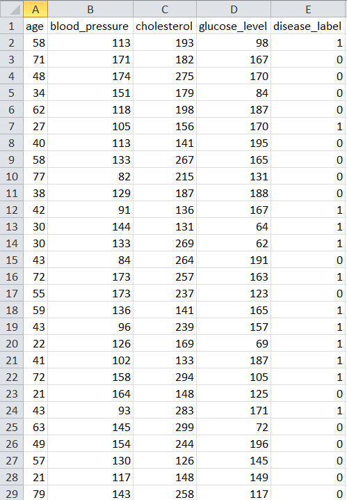
We gather the synthetic medical data to mimic a practical scenario in this step. The historical data is available in CSV file format. The data includes random values for features like “age”, “blood_pressure”, “cholesterol”, and “glucose_level”. The corresponding binary “disease_label” (0 or 1) represents the absence or presence of a disease. The data is saved in the “medical_data.csv” file. Here is the sample data snapshot:

Step 5: Load and Preprocess the Data

In this step, load the previously collected synthetic data from the CSV file (medical_data.csv) using the Pandas library. To prepare the DataFrame for machine learning, we extract the features and labels. Data preprocessing, which includes duties like addressing missing values, scaling features, or one-hot encoding categorical variables, is frequently performed after this phase. We omit the data preprocessing in this case because the synthetic data is generated without missing values or categorical attributes.

Code Snippet:

medical_disease_data = pd_obj.read_csv('medical_data.csv')

# Extract features (age, blood_pressure, cholesterol, glucose_level) and labels (disease_label)

features = medical_disease_data[['age', 'blood_pressure', 'cholesterol', 'glucose_level']].values

labels = medical_disease_data['disease_label'].values

Step 6: Splitting the Data into Testing and Training Sets

To evaluate the effectiveness of the MLM (Machine Learning Model), we need to separate the data into training sets and testing sets with the assistance of the train_test_split function of the sci-kit-learn library. The model is trained using 70% of the data from the training set, and its performance is assessed using 30% of the data from the testing set.

train_features, test_features, train_labels, test_labels = tts(test_size=0.3, features, labels, random_state=40)

Step 7: Define the Neural Network Model

Using the Keras API of TensorFlow, define a basic neural network model in this stage. Three dense layers make up the model. The “relu” activation function is used by the 64 and 32 neurons in the first two layers, respectively. Since the task requires binary classification, the final layer contains a single neuron with a “sigmoid” activation function.

nerual_Network_Model = tf.keras.Sequential([

tf.keras.layers.Dense(64, activation='relu', input_shape=(4,)),

tf.keras.layers.Dense(32, activation='relu'),

tf.keras.layers.Dense(1, activation='sigmoid')

])

Step 8: Compile the NN (Neural Network) Model

It must be assembled before the model can be trained. We employ the well-known “adam” optimizer that is used in gradient-based optimization techniques by employing the “binary_crossentropy” method as the loss function for binary classification since it works well with models that provide probabilities. Additionally, we list the “accuracy” as the measure to monitor while training.

nerual_Network_Model.compile(loss= 'binary_crossentropy', optimizer='adam', metrics= ['accuracy'])

Step 9: Perform Model Training on the Medical Data

To use the historical data to train the neural network model, use the code that accepts the features and labels: the number of epochs (10 in this case), the batch size (32 in this example), the training features and labels, as well as the validation data (the testing features and labels). According to the epochs argument, the model is trained on the full training dataset in a specified number of times. The number of samples that is used to train the model at one time is determined by the batch_size argument. A dataset that is used to assess the model’s performance during training is specified by the validation_data argument.

nerual_Network_Model.fit(epochs=10, train_features, train_labels, batch_size=32, validation_data=(test_features, test_labels))

Step 10: Estimate the NN Model on the Basis of the Test Dataset

After the successful model training phase, we now apply the evaluate technique to assess and estimate its performance based on the test dataset. After that, the test accuracy is printed to the console.

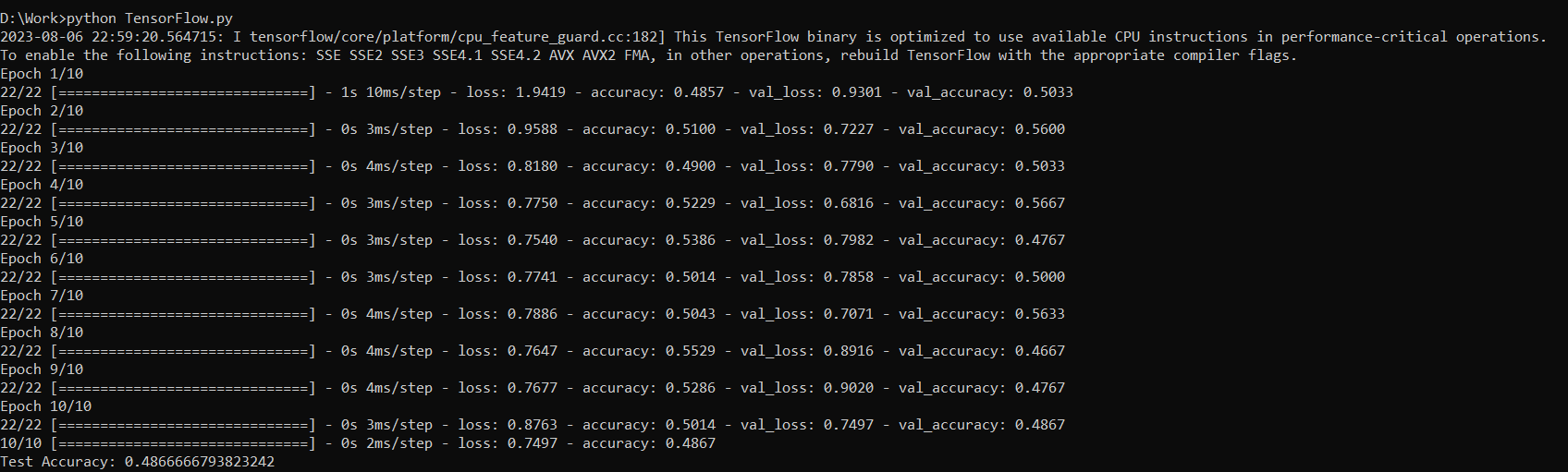
test_loss, nerual_test_accuracy = nerual_Network_Model.evaluate(test_features, test_labels)

Step 11: Run the Code Using Python

Executing the code using the Python compiler is the last step. Launch the command prompt, then type “Python” and the file name with the “.py” extension. Introducing TensorFlow allows the model’s accuracy to vary on each run. Here is the code’s sample output on each run:

Limitations to Use TensorFlow

Complexity: TensorFlow is challenging to understand and implement, especially for those who are just starting with machine learning tools.
Performance: TensorFlow is extremely slow for particular workloads, including inference on mobile devices.
Dependencies: TensorFlow depends on a number of other libraries which can make it difficult to install and use.
Storage: It takes extra space for installation.

Conclusion

Overall, TensorFlow is a powerful and versatile framework for deep learning (DL) and machine learning (ML). It is a good choice for organizations that need a flexible and scalable framework for solving various problems.