Before drinking wine, it is good to check the quality and chemical quantity that is added in your wine. We will help you to predict the quality of your wine (low, medium, and high) using Machine Learning through Python. In this guide, we will discuss the attributes that are included in wine and estimate the wine quality based on these. Five different classification algorithms are implemented in this guide.
Features
The following are some attributes that we will consider while predicting the quality of wine:
- alcohol: This attribute specifies the percent of alcohol that is present in the wine. Most of the wines hold 2 – 8 percent alcohol in ot.
- pH: This attribute holds the pH value of the wine. Typically, the pH level of a wine ranges from 3 to 4.
- residual sugar: All wines go through the fermentation process. After this process, some sugar are left. This is known as residual sugar.
- chlorides: This is the salt content that is present in the wine.
- citric acid: This is added in wines to make it citric and it is of organic acid type which is weak.
- fixed acidity: Tartaric acid, malic acid, and citric acid are the fixed acids that are fixed in wine.
- Sulphates: These are added to wine to get rid of bacteria and keep the wine fresh.
Implementation
In Machine Learning, if you are working with categorical data, you need to understand the Classification. Classification is a Supervised Learning Technique in Machine Learning which is used to identify the category of the new observations.
Loading the Data
Download this dataset (wine_data.csv) from here.
The read_csv() is the available function in the Pandas module that is used to load the CSV data into a variable. It takes the file name as the parameter.
- After the load, display the DataFrame after loading the data. Then, we use the pandas.DataFrame.shape attribute to display the total number of rows and columns that are present in the DataFrame. It returns a tuple of values. The first value refers to the total number of rows and the second value refers to the total number of columns/attributes.
- Also, display all the columns using the “pandas.DataFrame.columns” attribute.
- Use the pandas.DataFrame.head() function to display the first three records.
# Load the wine_data.csv into the train_data variable
train_data=pandas.read_csv('wine_data.csv')
# Get the dimensionality of the train_data
print(train_data.shape,"\n")
# Get the column names
print(train_data.columns,"\n")
# Top 3 rows
print(train_data.head(3))
Output:

So, our dataset holds 6497 records and 13 columns.
Data Cleaning
In this stage, we can get rid of the missing values if they exist. Use the pandas.DataFrame.isnull().sum() function to get the count of missing values from the entire DataFrame.
print(train_data.isnull().sum())
Output:
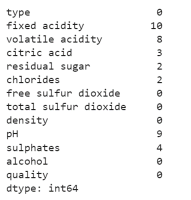
The missing values exist in the seven columns [“fixed acidity”, “volatile acidity”, “citric acid”, “residual sugar”, “chlorides”, “pH”, “sulphates”].
The DataFrame[‘column_name’].fillna(DataFrame[‘column_name’].mean()) is used to replace the missing values with the mean in the specific column.
train_data['fixed acidity']= train_data['fixed acidity'].fillna(train_data['fixed acidity'].mean())
train_data['volatile acidity']= train_data['volatile acidity'].fillna(train_data['volatile acidity'].mean())
train_data['citric acid']= train_data['citric acid'].fillna(train_data['citric acid'].mean())
train_data['residual sugar']= train_data['residual sugar'].fillna(train_data['residual sugar'].mean())
train_data['chlorides']= train_data['chlorides'].fillna(train_data['chlorides'].mean())
train_data['pH']= train_data['pH'].fillna(train_data['pH'].mean())
train_data['sulphates']= train_data['sulphates'].fillna(train_data['sulphates'].mean())
train_data.describe()
Output:
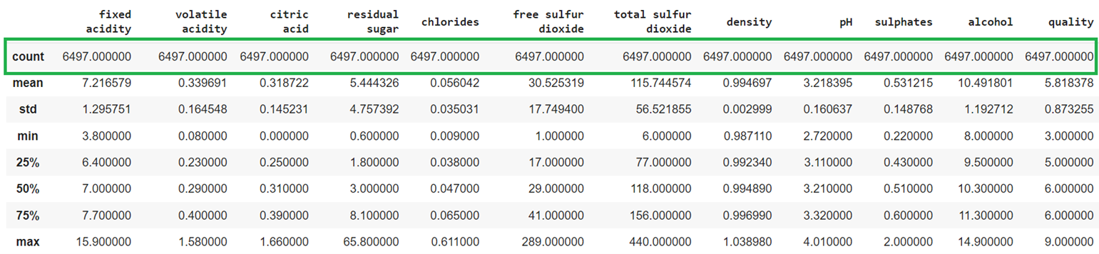
Now, the missing values do not exist in the DataFrame.
Data Visualization
Use the hist() function to view the Histograms for the numeric type (int64, float64) columns.
train_data.hist(color='green',figsize=(10,10))
Output:
Histogram is generated for the following attributes:

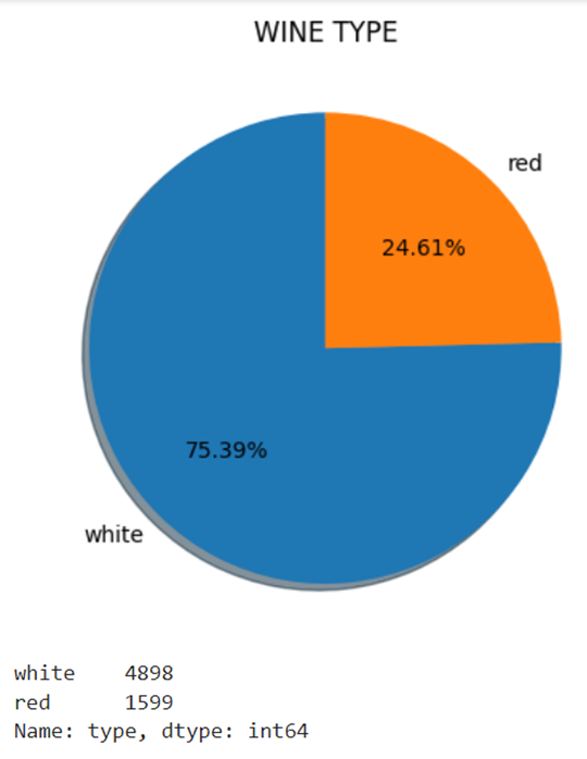
Create a Pie chart to get all the categories that are present in the column type. We can create it using the pyplot. After that, use the value_counts() function to get the count of values that are present in each category.
# Create Pie chart
pyplot.pie(train_data['type'].value_counts().reset_index()['type'], labels=train_data['type'].value_counts().reset_index()['index'], autopct='%1.2f%%',shadow = True, startangle = 90)
# Set the title to the Pie chart
pyplot.title('WINE TYPE')
# Display the Pie chart
pyplot.show()
# Get the count for each category
print(train_data['type'].value_counts())
Output:
There are two categories in the smoking_status column.
- white – 4898
- red – 1599
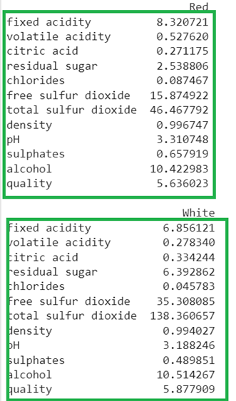
Get the red wine and white wine from the train_data with the average value of all the columns.
red_wine = pandas.DataFrame({"Red" : train_data[train_data["type"] == "red"].describe().loc["mean"]})
print(red_wine,"\n")
# Get the white wine from the train_data with the average value of all the columns.
red_wine = pandas.DataFrame({"White" : train_data[train_data["type"] == "white"].describe().loc["mean"]})
print(red_wine)
Output:
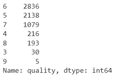
Return the count of values for each category in the quality column using the pandas.DataFrame.value_counts() function.
print(train_data['quality'].value_counts())
Output:
The total number of categories is 7.
Use the “seaborn” module and plot the alcohol and quality columns using the barplot.
seaborn.barplot(x= 'quality', y = 'alcohol', data = train_data)
Output:

Quality vs citric acid
seaborn.barplot(x= 'quality', y = 'citric acid', data = train_data)
Output:

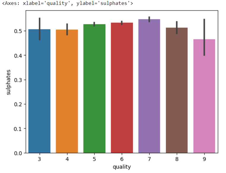
Quality vs sulphates
seaborn.barplot(x= 'quality', y = 'sulphates', data = train_data)
Output:
Data Transformation
The pandas.DataFrame[‘column_name’].replace({‘existing’:new,……}) is used here. It takes a dictionary of values in which the key is the existing categorical elements and the value is the numeric value that updates the key.
- Let’s convert all the categorical elements to categorical numeric values in the column type.
- Also, we segregate seven categories into three categories in the quality column. This will help us to predict the wine much easier.
train_data['type'] = train_data['type'].replace({'red':0,'white':1})
# Replace 3 and 4 with 0,
# 5,6,and 7 with 1 and
# 8,9 with 2.
train_data['quality'] = train_data['quality'].replace({3 : 0,4 : 0, 5 : 1, 6 : 1, 7 : 1, 8 : 2, 9 : 2})
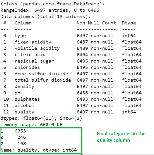
train_data.info()
train_data['quality'].value_counts()
Output:
Now, you can see that all the column types are now numeric and the total categories in the quality column is 3 instead of 7.
Preparing the Train and Test Data
It is a good practice to separate the data for training and testing within the given dataset that is used for training. For example, if the training dataset holds 100 records, 70 records are used to train the Machine Learning Model and 30 records are used to test the model (Prediction). The train_test_split() method automatically splits the dataset into the Train data and Test data. It is available in the sklearn.model_selection module. Basically, the train_test_split() takes five parameters.
- The Training_set is the actual dataset with independent attributes.
- The target represents the class label (dependent attribute).
- The test_size takes a decimal value which represents the size of the data from the Training_set that is used for testing. For example, if it takes 0.3, 30% of the Training_set is used for testing.
- The random_state is used to fetch the records for testing. If it is 0, every time the same records are taken for testing. This parameter is optional
- If you don’t want to shuffle the Training_set before splitting, you can set this parameter to False.
It returns the Training_Independant_Attribtes, Training_target, Testing_Independant_Attribtes, and Testing_target.
In our case, “quality” is the class label/target. Let’s store it in the target variable and drop it from the train_data. Then, split the data – Testing: 30% and Training: 70%.
# Store the quality column values in a target variable
target = train_data['quality']
# Include the independent attributes by dropping the target attribute
train_data = train_data.drop(['quality'], axis=1)
# Split the train_data into the train and test sets
X_train, X_test, y_train, y_test = train_test_split(train_data,target,test_size=0.3)
print(X_train.shape)
print(X_test.shape)
Output:
After splitting the train_data, out of 6497 records, 4547 records are used for training and 1950 records are used for testing the model.

Model Fitting and Evaluation
- Import the model from the specific module.
- Define the model.
- Fit the model using the fit() method. It takes the Training – Independent data as the first parameter and the Training – Target data as the second parameter.
- Predict the model for the records that are used for testing (test the independent attributes). The predict() function takes the array of records to be predicted.
- Finally, use the score() function to get the model1 accuracy. It takes the Testing – Independent data as the first parameter and the Testing – Target data as the second parameter.
For all the models, we use the same record to predict the wine quality.
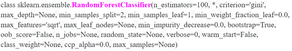
RandomForestClassifier
Let’s build a model with “RandomForestClassifier” and display the score of this model. We can pass the following parameters to this model. Now, we are not passing n_estimators as 100; the criterion type is “gini” and the bootstrap is set to True:
# Define the model with 100 trees
model1 = RandomForestClassifier(n_estimators=100,criterion="gini",bootstrap=True)
# Fit the model
model1.fit(X_train, y_train)
# model1 score
print(model1.score(X_test,y_test) * 100)
Output:
[1]
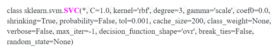
SVC
Let’s build a model with Support Vector Classification from Support Vector Machine and display the score of this model. We can pass the following parameters to this model. But now, we are not passing any parameters to the model:
# Define the SVC model.
model2 = svm.SVC()
# Fit the model
model2.fit(X_train, y_train)
# model2 score
print(model2.score(X_test,y_test) * 100)
# Test record to predict the wine quality
test_record=[1,5.8,0.28,0.27,2.6,0.054,30,156,0.9914,3.53,0.42,12.4]
print(model2.predict([test_record]))
Output:
[1]
ExtraTrees Classifier
Let’s build a model with ExtraTreesClassifier. It can be imported from the “sklearn.ensemble” module. As of now, we are not passing any parameters to the model.
# Define the model
model3 = ExtraTreesClassifier()
# Fit the model
model3.fit(X_train, y_train)
# model3 score
print(model3.score(X_test,y_test) * 100)
# Test record to predict the wine quality
test_record=[1,5.8,0.28,0.27,2.6,0.054,30,156,0.9914,3.53,0.42,12.4]
print(model3.predict([test_record]))
Output:
[1]
Bagging Classifier
Let’s build a model with BaggingClassifier by passing the RandomForestClassifier as the estimator.

# Define the model
model4 = BaggingClassifier(estimator=model1, n_estimators=10,)
# Fit the model
model4.fit(X_train, y_train)
# model4 score
print(model4.score(X_test,y_test) * 100)
# Test record to predict the wine quality
test_record=[1,5.8,0.28,0.27,2.6,0.054,30,156,0.9914,3.53,0.42,12.4]
print(model4.predict([test_record]))
Output:
[1]
Voting Classifier
Now, pass all the previous models to the Voting Classifier as estimators with the hard voting parameter.
# Define the model
model5 = VotingClassifier(estimators=[('Random Forest',model1),('Extra Trees',model2),('Support Vector Machine',model3),('Bagging',model4)],voting="hard")
# Fit the model
model5.fit(X_train, y_train)
# model5 score
print(model5.score(X_test,y_test) * 100)
# Test record to predict the wine quality
test_record=[1,5.8,0.28,0.27,2.6,0.054,30,156,0.9914,3.53,0.42,12.4]
print(model5.predict([test_record]))
Output:
[1]
We can see that for all five models, the accuracy is closer and all the predicted results are the same.
Conclusion
Now, you are able to predict the quality of wine using the Machine Learning Technology. In this guide, we considered the dataset that holds two types of wine (red and white) with different chemicals. The Classification technique is used to predict the quality of wine by segregating seven categories into three categories. This improved the model accuracy and now we can predict any kind of record. Also, we learned about the five different models to predict the quality of wine.