In today’s world, we are seeing unusual rain. Due to this, the Agriculture sector is one of the more impacting sectors due to floods and unnecessary water content for the crops. If we predict the rainfall prior to the irrigation, we can save the crops and also some crops that need more water content. So, these types of crops are planted at this moment. In this guide, we will discuss how to predict whether the rain will occur on the next day or not (Yes/No) using Machine Learning through Python. We will consider Australia’s rainfall dataset for this prediction. Also, this is a larger dataset. So, the Random Forest (Ensembling Technique) is utilized to train our model.
Classification
In Machine Learning, if you are working with categorical data, you need to understand Classification. Classification is a Supervised Learning Technique in Machine Learning which is used to identify the category of the new observations.
For example, in our scenario, the independent attributes are temperature, humidity, windy, and sunshine, evaporation, etc. We are only able to predict the rainfall based on these. So, these are the independent attributes which do not depend on anything. Rainfall (Yes/No) is the target attribute or class label which depends upon these attributes.
Ensembling Technique
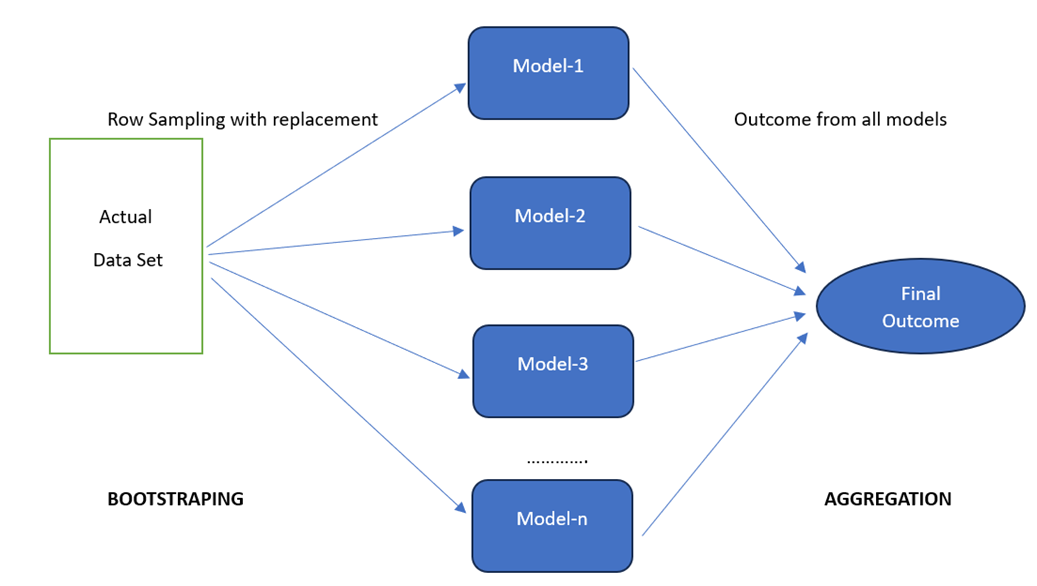
Ensembling means combining multiple models. We will train the dataset samples with each model and combine the outcome of all the models. Bagging is one of the Ensembling Techniques.
Bagging is also known as BootStrap Aggregation in which we combine multiple models. These are known as “Weak Learners”. For each of them, we need to provide a sample data (D1,D2,…Dn) from the existing dataset (D) such that D1<D, D2<D,… This is known as “Row Sampling” with replacement. Finally, we combine all the outcomes from all the models. This is known as “Aggregation”. This can be done using the Voting Classifier. The majority of the outcome will be the final outcome.
Random Forest
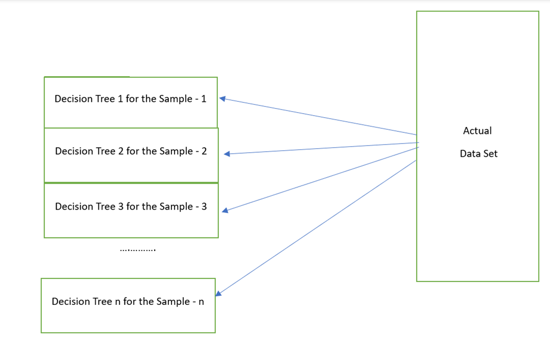
Random Forest is one of the Bagging Techniques which performs the same functionality that is similar to Decision Tree. But it takes a Forest (collection of Decision Trees) and combine (maximum outcome) all the outputs of the Decision Trees. For example, if the Random Forest size is 3, internally three Decision Trees are created and the rainfall outcome of the first and second Decision Trees are “Yes” and the last tree is “No”. It considers “Yes” since it is the maximum outcome.
In Python, the “RandomForestClassifier” is available in the “sklearn.ensemble” module. The following is the model with parameters. We use only some parameters to build our model. So, we will discuss only those parameters.
Syntax:
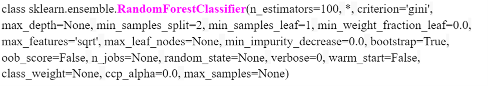
- We can specify the number of trees in the “n_estimators” parameter. It is 100 by default.
- By default, bootstrap is True. As we discussed in Emsemblign, bootstrap splits the dataset into samples while building the Decision Trees in the Random Forest. The entire dataset is used to build each tree when it is set to False.
- If the bootstrap is set to True, the “max_samples” parameter takes the number of samples to draw from X to train the each base estimator.
Implementation
Let’s predict if the rainfall will occur tomorrow or not using the weather conditions like cloud, wind, temperature, humidity, etc. We will consider the outdoor_games (CSV file) dataset with 14 records (used to train and test the Machine Learning model).
Loading the Data
Pandas is a module that is available in Python which is used for data analysis. We utilize this module to load the datasets into the Python environment. Here, we use the Google Colab as the code environment. This is available for free. Just a Google account is needed.
First, we need to load the file from our local PC to the Colab Env. Download this dataset (Rainfall_dataset.csv) from here.
from google.colab import files
files.upload()

The read_csv() is the available function in the Pandas module that is used to load the CSV data into a variable. It takes the file name as the parameter. After the load, display the DataFrame after loading the data. Then, we use the shape attribute to display the total number of rows and columns that are present in the DataFrame. It returns a tuple of values. The first value refers to the total number of rows and the second value refers to the total number of columns/attributes.
# Load the Rainfall_dataset.csv into the train_data variable
train_data=pandas.read_csv('Rainfall_dataset.csv')
# Get the dimensionality of the train_data
train_data.shape
Output:
Our dataset holds 1,45,460 records/rows and 23 columns.
(145460, 23)
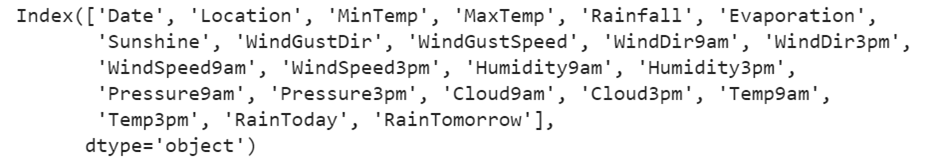
You can get all the column using the “pandas.DataFrame.columns” attribute.
Output:
Data Preprocessing
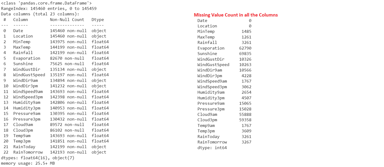
Now, we have the data (train_data). Data preprocessing is the important step in this guide to deal with missing values that are present in our dataset. You will lose the model accuracy if the dataset holds the NaN values. So, we need to remove/replace them with other values. We first see how many missing values exist in all the columns and then replace them with the mean of the column (Numeric Type column) values.
# Get the Null value count in all the columns of the train_data
print(train_data.isnull().sum())
Output:
The first output holds all the columns with non-null values: Count and Datatype. The second output displays the total count of missing values in all the columns.
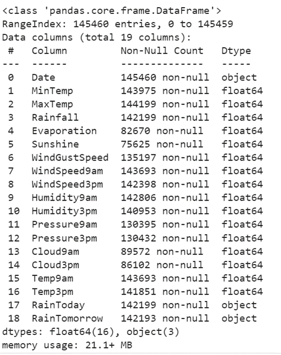
Now, we need to remove unwanted columns from the train_data. Let’s remove these columns [“WindGustDir”, “Location”, “WindDir9am”, “WindDir3pm”] using the drop() function.
train_data= train_data.drop(["WindGustDir", "Location", "WindDir9am","WindDir3pm"], axis=1)
print(train_data.info(),"\n")
Output:
Now, these three columns don’t exist in the DataFrame.
Now, we can replace the missing values (NaN) with the mean of the existing column values. The DataFrame[‘column_name’].fillna(DataFrame[‘column_name’].mean()) is used to replace the missing values with the mean in the specific column. The columns are [MinTemp, MinTemp, Rainfall, Evaporation, Sunshine, WindGustSpeed, WindSpeed9am, WindSpeed3pm, Humidity9am, Humidity3pm, Pressure9am, Pressure3pm, Cloud9am, Cloud3pm, Temp9am and Temp3pm].
train_data['MaxTemp']=train_data['MaxTemp'].fillna(train_data['MaxTemp'].mean())
train_data['MinTemp']=train_data['MinTemp'].fillna(train_data['MinTemp'].mean())
train_data['Rainfall']=train_data['Rainfall'].fillna(train_data['Rainfall'].mean())
train_data['Evaporation']=train_data['Evaporation'].fillna(train_data['Evaporation'].mean())
train_data['Sunshine']=train_data['Sunshine'].fillna(train_data['Sunshine'].mean())
train_data['WindGustSpeed']=train_data['WindGustSpeed'].fillna(train_data['WindGustSpeed'].mean())
train_data['WindSpeed9am']=train_data['WindSpeed9am'].fillna(train_data['WindSpeed9am'].mean())
train_data['WindSpeed3pm']=train_data['WindSpeed3pm'].fillna(train_data['WindSpeed3pm'].mean())
train_data['Humidity9am']=train_data['Humidity9am'].fillna(train_data['Humidity9am'].mean())
train_data['Humidity3pm']=train_data['Humidity3pm'].fillna(train_data['Humidity3pm'].mean())
train_data['Pressure9am']=train_data['Pressure9am'].fillna(train_data['Pressure9am'].mean())
train_data['Pressure3pm']=train_data['Pressure3pm'].fillna(train_data['Pressure3pm'].mean())
train_data['Cloud9am']=train_data['Cloud9am'].fillna(train_data['Cloud9am'].mean())
train_data['Cloud3pm']=train_data['Cloud3pm'].fillna(train_data['Cloud3pm'].mean())
train_data['Temp9am']=train_data['Temp9am'].fillna(train_data['Temp9am'].mean())
train_data['Temp3pm']=train_data['Temp3pm'].fillna(train_data['Temp3pm'].mean())
print(train_data.info(),"\n")
Output:
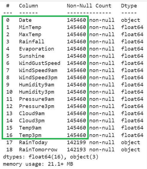
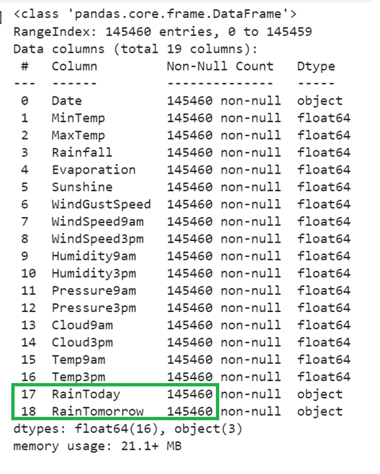
Still, the missing values exist in the “RainToday” and “RainTomorrow” columns. Also, they are of Object type. We need to convert the categorical elements into categorical numeric values. Let’s get the unique categorical elements from these two columns using the value_counts() function.
print(train_data['RainToday'].value_counts(),"\n")
# Get the unique elements from the RainTomorrow column
print(train_data['RainTomorrow'].value_counts(),"\n")
Output:
There are only two categorical elements in both the columns (Yes and No).
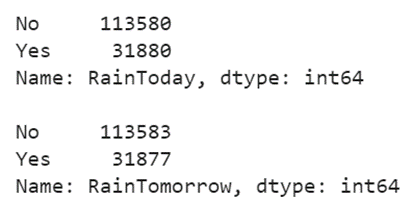
The maximum count of “No” is high. So, replace the missing values with “No” in both these columns.
train_data['RainTomorrow']=train_data['RainTomorrow'].fillna('No')
print(train_data.info(),"\n")
Output:
Now, the missing values are removed from the DataFrame.
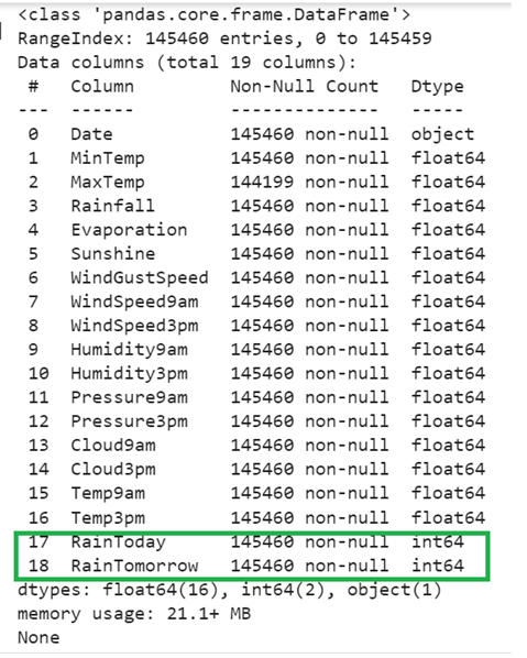
Let’s convert all the categorical elements to categorical numeric values in each column using the pandas.DataFrame[‘column_name’].replace({‘existing’:new,……}). It takes a dictionary of values in which the key is the existing categorical elements and value is the numeric value that updates the key. Here, we do it for two columns – “RainToday” and “RainTomorrow”. Replace “No” with 0 and “Yes” with 1.
train_data['RainToday']=train_data['RainToday'].replace({'No':0,'Yes':1})
train_data['RainTomorrow']=train_data['RainTomorrow'].replace({'No':0,'Yes':1})
print(train_data.info(),"\n")
Output:
Feature Extraction
The “Date” column exists in the DataFrame. It is good to extract the day, year, and month from it into new columns. So, extracting features is known as “Feature Extraction”. We need to convert the “Date” column that is present in the train_data into the Pandas Date using the pandas.to_datetime() function. After that, we can extract the “Date” attributes.
- Use the “dt.day” attribute to extract the day from the “Date” column and store it in the “Day” column.
- Use the “dt.month” attribute to extract the month from the “Date” column and store it in the “Month” column.
- Use the “dt.year” attribute to extract the year from the “Date” column and store it in the “Year” column.
# Extract the Day from the Date into the Day column
train_data['Day']=train_data["Date"].dt.day
# Extract the Month from the Date into the Month column
train_data['Month']=train_data[ "Date"].dt.month
# Extract the Year from the Date into the Year column
train_data['Year']=train_data[ "Date"].dt.year
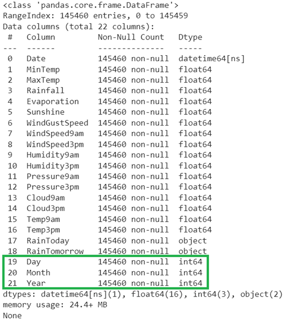
print(train_data.info(),"\n")
Output:
Now, we have extra three columns in the DataFrame.
Preparing the Train and Test Data
It is a good practice to separate the data for training and testing within the given dataset that is used for training. For example, if the Training dataset holds 100 records, 70 records are used to train the Machine Learning Model and 30 records are used to test the model (Prediction). The train_test_split() method automatically splits the dataset into Train data and Test data. It is available in the “sklearn.model_selection” module. Basically, the train_test_split() takes five parameters.
- The Training_set is the actual dataset with independent attributes.
- The target represents the class label (dependent attribute).
- The test_size takes a decimal value which represents the size of data from the Training_set that is used for testing. For example, if it takes 0.3, 30% of the Training_set is used for testing.
- The random_state is used to fetch the records for testing. If it is 0, every time the same records are taken for testing. This parameter is optional.
- If you don’t want to shuffle the Training_set before splitting, you can set this parameter to False.
It returns the Training_Independant_Attribtes, Training_target, Testing_Independant_Attribtes, and Testing_target.
In our case, “RainTomorrow” is the class label/target. Let’s store it in the target variable and drop it from the train_data. Then, split the data – Testing: 30% and Training: 70%.
# Store RainTomorrow column values in a target variable
target = train_data['RainTomorrow']
# Include the independent attributes by dropping 'RainTomorrow' and 'Date' by dropping columns.
train_data = train_data.drop(['RainTomorrow', 'Date'], axis=1)
# Split the train_data into the train and test sets
X_train, X_test, y_train, y_test = train_test_split(train_data,target,test_size=0.3)
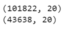
print(X_train.shape)
print(X_test.shape)
Output:
After splitting the train_data, out of 1,45,460 records, 1,01,822 records are used for training and 43,638 records are used for testing the model.
Model Fitting and Evaluation – Random Forest
- Import the DecisionTreeClassifier from the “sklearn.tree” module.
- Define the RandomForestClassifier Model – model1 with parameters – n_estimators=50, criterion=”gini”, bootstrap=True and max_samples=20.
- Fit the model using the fit() method. It takes the Training – Independent data as the first parameter and the Training – Target data as the second parameter.
- Predict the model1 for the records that are used for testing (test the independent attributes). The predict() function takes the array of records to be predicted.
- Finally, use the score() function to get the model1 accuracy. It takes the Testing – Independent data as the first parameter and the Testing – Target data as the second parameter.
# Define the model with 50 trees
model1 = RandomForestClassifier(n_estimators=50,criterion="gini",bootstrap=True,max_samples=20)
# Fit the model
model1.fit(X_train, y_train)
# Predict the data and get the model score
y_pred = model1.predict(X_test)
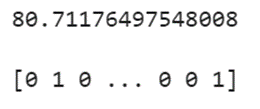
print(model1.score(X_test,y_test) * 100,"\n")
print(y_pred)
Output:
The model score is 80.711%.
Let’s fit a model using the DecisionTreeClassifier.
# Define the model
model2 = DecisionTreeClassifier()
# Fit the model
model2.fit(X_train, y_train)
# Predict the data and get the model score
y_pred = model2.predict(X_test)
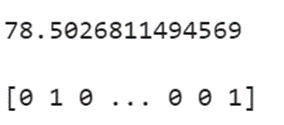
print(model2.score(X_test,y_test) * 100,"\n")
print(y_pred)
Output:
If you try with the Decision Tree, it gives only 78.5% accuracy.
Conclusion
We learned now how to predict the rainfall that will occur the next day or not using one of the Machine Learning Classification – Ensembling Technique (Random Forest). Also, we fitted a model using the Decision Tree but is given less accuracy than the Random Forest. Also, this dataset includes the data preprocessing steps like Data Cleaning (missing values removal from the specific columns) and Data Transformation. Each step is explained with code snippets and outputs.