The weather (temperature, humidity, etc.) affects almost everything we do in our daily lives. For example, tomorrow a volleyball match is scheduled in your area and suddenly the wind is heavy and you are unable to play the match. All the setup and preparations are useless and may also lose the budget that is supposed to be spent for the day. In these scenarios, if you predict the weather conditions, you will save time and get rid of wasting the budget. In this guide, we will see how to predict if the volleyball (outdoor) game is played on a particular day or not based on the weather conditions using Machine Learning.
Classification:
In Machine Learning, if you are working with categorical data, you need to understand Classification. Classification is a Supervised Learning Technique in Machine Learning which is used to identify the category of the new observations.
For example, in our scenario, the independent attributes are outlook, humidity, windy, and temperature. Based on these, we are able to predict the weather and play the outdoor games. So, these are the independent attributes which do not depend on anything. Play (Yes/No) is the target attribute or class label which depends upon these attributes.
Decision Tree
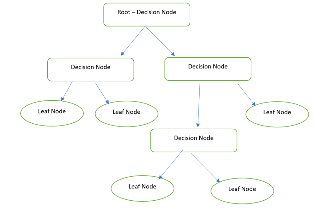
Basically, the Decision Tree is a graphical representation to get all the possible solutions to a problem based on the provided conditions using nodes. The Decision node is used to make the decision and the Leaf node refers to the output of a specific decision.
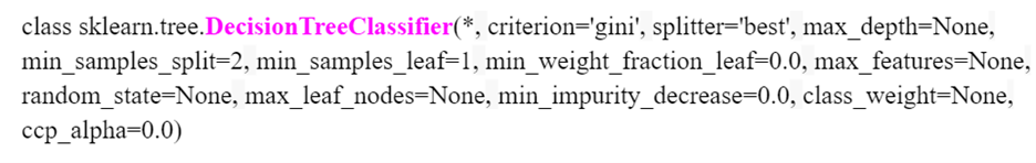
In Python, the DecisionTreeClassifier is available in the “sklearn.tree” module. We will see how to specify this while implementing the project. The following is the model with parameters.
Syntax:
We will not pass any parameter while defining the model. There are possible parameters that we can pass to this model.
Random Forest
Random Forest performs the same functionality as the Decision Tree. But it takes a Forest (collection of Decision Trees) and combine (maximum outcome) all the outputs of the Decision Trees. For example, a random Forest size is 3. So, internally, three Decision Trees are created and the Play outcome of the first and second Decision Trees are “Yes” and the last tree is “No”. It considers “Yes” since it is the maximum outcome.
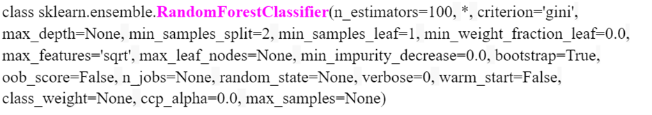
In Python, the RandomForestClassifier is available in the “sklearn.ensemble” module. The following is the model with parameters. We can specify the number of trees in the “n_estimators” parameter. It is 100 by default.
Syntax:
Implementation:
Let’s predict whether we play volleyball or not. We will consider the outdoor_games (CSV file) dataset with 14 records (used to train and test the Machine Learning model).
Loading the Data
Pandas is a module that is available in Python which is used for data analysis. We will utilize this module to load the datasets into the Python environment. Here, we use the Google Colab as the code environment. This is available for free. Just a Google account is needed.
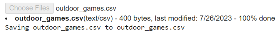
First, we need to load the file from our local PC to the Colab Env. Download this dataset from here.
from google.colab import files
files.upload()
The read_csv() is the function that is available in the Pandas module which is used to load the CSV data into a variable. It takes the file name as the parameter. After the load, display the DataFrame after loading the data.
# Load the outdoor_games.csv into the train_data variable
train_data=pandas.read_csv('outdoor_games.csv')
# Display
train_data
Output:
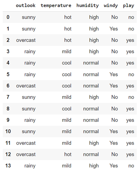
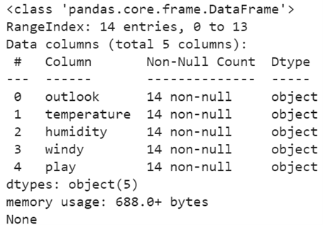
There are five attributes in this DataFrame. “Outlook”, “temperature”, “humidity”, and “windy” are independent attributes and “play” is the target attribute (class label) that depends upon these independent attributes. Let’s get the column names separately with data types. The pandas.DataFrame.info() is used to get this information.
Output:
All the five attributes are objects. We need to convert them into categorical – numeric forms because the machines will not understand the objects.
Data Preprocessing
In this phase, we will first see the categorical values in each column and then convert them into categorical numeric values.
The pandas.DataFrame[‘column_name’].value_counts() is utilized to get all the unique categorical elements from the specified column. It also displays the total occurrence of each categorical value.
print(train_data['outlook'].value_counts(),"\n")
print(train_data['temperature'].value_counts(),"\n")
print(train_data['humidity'].value_counts(),"\n")
print(train_data['windy'].value_counts(),"\n")
print(train_data['play'].value_counts())
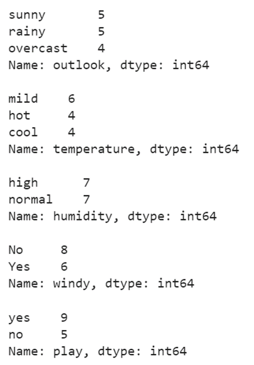
Output:
- In the outlook column, there are three categorical elements: “sunny”, “rainy”, and “overcast”.
- In the temperature column, there are three categorical elements: “mild”, “hot”, and “cool”.
- In the humidity column, there are two categorical elements: “high” and “normal”.
- In the windy column, there are two categorical elements: “No” and “Yes”.
- In the play column, there are two categorical elements: “no” and “yes”.
Let’s convert all the categorical elements to categorical numeric values in each column using the pandas.DataFrame[‘column_name’].replace({‘existing’:new,……}). It takes a dictionary of values in which the key is the existing categorical elements and the value is the numeric value that updates the key. Let’s replace the categorical elements with categorical numeric values in all five attributes one after another.
train_data['outlook']=train_data['outlook'].replace({'sunny':0,'rainy':1,'overcast':2})
# Replace 'mild' with 0,'hot' with 1,'cool' with 2 in the temperature attribute
train_data['temperature']=train_data['temperature'].replace({'mild':0,'hot':1,'cool':2})
# Replace 'high' with 0,'normal' with 1 in the humidity attribute
train_data['humidity']=train_data['humidity'].replace({'high':0,'normal':1})
# Replace 'No' with 0,'yes' with 1 in the windy attribute
train_data['windy']=train_data['windy'].replace({'No':0,'Yes':1})
# Replace 'no' with 0,'yes' with 1 in the play attribute
train_data['play']=train_data['play'].replace({'no':0,'yes':1})
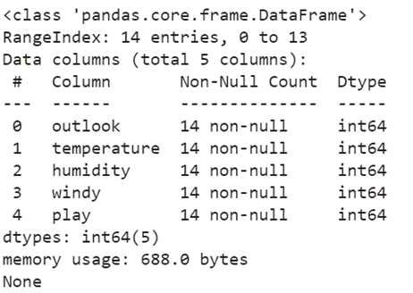
print(train_data.info())
Output:
Now, all attributes are of Integer (int64) type.
Preparing the Train and Test Data
It is a good practice to separate the data for training and testing within the given dataset used for training. For example, if the training dataset holds 100 records, 70 records are used to train the Machine Learning Model and 30 records are used to test the model (Prediction). The train_test_split() method automatically splits the dataset into the Train data and Test data. It is available in the “sklearn.model_selection” module. Basically, the train_test_split() takes five parameters.
- The Training_set is the actual dataset with independent attributes.
- The target represents the class label (dependent attribute).
- The test_size takes a decimal value which represents the size of the data from the Training_set that is used for testing. For example, if it takes 0.3, 30% of the Training_set is used for testing.
- The random_state is used to fetch the records for testing. If it is 0, every time the same records are taken for testing. This parameter is optional
- If you don’t want to shuffle the Training_set before splitting, you can set this parameter to False.
It returns the Training_Independant_Attribtes, Training_target, Testing_Independant_Attribtes and Testing_target.
In our case, “play” is the class label/target. Let’s store it in the target variable and drop it from the train_data. Then, split the data – Testing: 20% and Training: 80%.
# Store the Class Label into the target variable
target=train_data['play']
# Drop the Class Label from the train_data
train_data=train_data.drop(['play'],axis=1)
# Split the train_data into Xtrain,Xtest,ytrain,ytest
Xtrain,Xtest,ytrain,ytest=train_test_split(train_data,target,test_size=0.2)
# Xtrain is used for training and ytrain represents the corresponding Class Label.
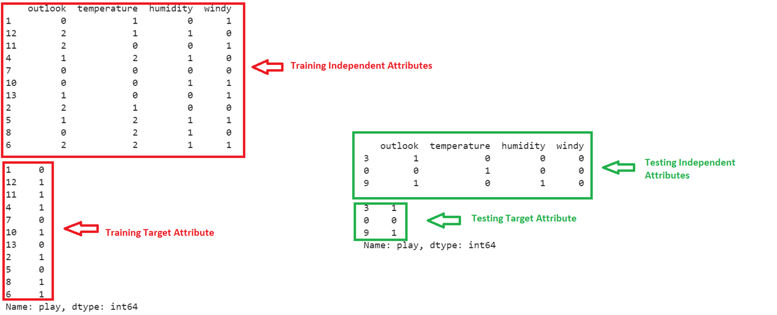
print(Xtrain,"\n")
print(ytrain,"\n")
# Xtest is used for testing and ytest represents the corresponding Class Label.
print(Xtest,"\n")
print(ytest)
Output:
After splitting the train_data, out of 14 records, 11 records are used for training and 3 records are used for testing the model.
Model Fitting and Evaluation – Decision Tree
- Let’s use the DecisionTreeClassifier to train the model.
- Import the DecisionTreeClassifier from the “sklearn.tree” module.
- Define the DecisionTreeClassifier – Model – model1.
- Fit the model using the fit() method. It takes the Training – Independent data as the first parameter and the Training – Target data as the second parameter.
- Predict the model1 for the records that are used for testing (test the independent attributes). The predict() function takes the array of records to be predicted.
- Finally, use the score() function to get the model1 accuracy. It takes the Testing – Independent data as the first parameter and the Testing – Target data as the second parameter.
Display the resulting Decision Tree using the plot_tree() function. We need to pass the model as the parameter to this function.
# Define the DecisionTreeClassifier - Model
model1=DecisionTreeClassifier()
# Fit the model
model1.fit(Xtrain,ytrain)
# Predict for the 3 records
print(model1.predict(Xtest),"\n")
# DecisionTreeClassifier - Model Score
print(model1.score(Xtest,ytest) * 100,"\n")
# Display the DecisionTree
from sklearn import tree
tree.plot_tree(model1)
Output:
Among three records, the first two records’ outcome is 0 which means that we are unable to play volleyball and the last outcome is 1 (we can play volleyball). The model score is 66% and you can view the Decision Tree.
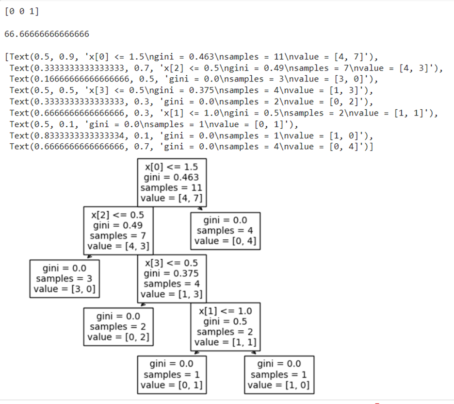
Output:
You are able to play the outdoor games with the Outlook as “overcast”, the Temperature as “hot”, the Humidity as “high”, and no wind.
Let’s use the RandomForestClassifier to train the model.
- Import the RandomForestClassifier from the “sklearn.ensemble” module.
- Define the RandomForestClassifier Model – model2. By default, 100 Decision Trees are created.
- Fit the model using the fit() method. It takes the Training – Independent data as the first parameter and the Training – Target data as the second parameter.
- Predict the model2 for the records that are used for testing (test the independent attributes). The predict() function takes the array of records to be predicted.
- Finally, use the score() function to get the model2 accuracy. It takes the Testing – Independent data as the first parameter and the Testing – Target data as the second parameter.
# Define the RandomForestClassifier - Model
model2=RandomForestClassifier()
# Fit the model
model2.fit(Xtrain,ytrain)
# Predict for the 3 records
print(model2.predict(Xtest),"\n")
# RandomForestClassifier - Model Score
print(model2.score(Xtest,ytest) * 100,"\n")
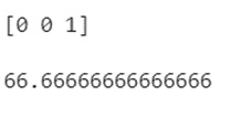
Output:
Among three records, the first two records’ outcome is 0 which means that we are unable to play volleyball and the last outcome is 1 (we can play volleyball). The model score is 66%.
Conclusion
Now, we can predict whether we can play the outdoor games or not using the Machine Learning algorithms based on the weather factors. The Classification Technique suits this scenario which categorizes the play status into Yes/No. In this guide, we discussed the two best algorithms (Decision Tree and Random Forest) and trained the model with these algorithms using Python. Each step is explained with code snippets and output. The data preprocessing is the important phase in this project to convert categorical items into categorical numeric values.