It’s a visual method of data analysis for summing up a single-variable dataset. Because the strip plot shows all of the observations as well as a depiction of the underlying distribution, it is considered reasonable to the box or violin plot.”
Syntax of the Stripplot in Seaborn
x, y, hue: To plot long-form data, you will need the inputs. These are the names of vector data or variables.
data: For plotting purposes, a data set has been created. The absence of x and y is read as wide-form. Aside from that, it’s likely to be long-form. A DataFrame in Pandas. However, defining the x, y, and hue parameters are necessary to easily specify how DataFrame data should be shown.
order, hue_order: For a gradient palette, this term includes the individual colors of each piece. The appropriate plot is returned by this method.
jitter: The extent of jitter that should be applied (just along the categorical axis). When you have many points that overlap, this can help you see the distribution more easily. You can either set the values of jitter (with the breadth of the uniformly distributed random variable range) or leave it at True as an acceptable default.
dodge: Enabling this to True when utilizing hue nesting separates the strips along the classified axis for distinct hue levels. Or else, each level’s points will be stacked on top of one another.
orient: The plot is oriented in a certain way (vertical or horizontal). This is normally inferred from the input variables’ types, but it can be utilized to clarify misunderstandings when both the parameters x and y are integers or when graphing wide-form data.
color: Color for all elements or a gradient palette’s seed.
palette: Colors to utilize for the hue variable’s various levels. Color palette() should be able to interpret it, or a dictionary relating hue values to matplotlib colors.
linewidth: The width of the grey lines that surround the plot points.
edgecolor: The color of the lines encircles each point. The brightness of the points is governed by the color palette used during the core of the points if you pass “grey.”
ax: The plot will be drawn onto the Axes object unless the current Axes object is used.
kwargs: Matplotlib.axes.Axes.scatter receives any additional keyword arguments().
Example 1
Here, we have a simple illustration of the strip plot with the seaborn module. Let’s get into the implementation part. We have set the style of the plot as darkgrid. The dataset mpg is imported inside the load_dataset(). Then, we have a strip plot function that has the x input as weight and y input as acceleration. This strip plot will compare the weight and acceleration of the mpg dataset. The code of seaborn stripplot is affixed here.
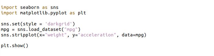
There we have got a basic visualization of the strip plot in the following graph figure.
Example 2
Here, we have a strip plot that is used to build a specific horizontal strip plot. When only one input parameter is used instead of two, the axis designates each of the input parameters as an axis. We have inserted the dataset tips in the load_dataset function. From the tips dataset, we have taken a column total_bills for our x input which is used in the strip plot function. The code of seaborn stripplot is affixed here.
The following figure shows the horizontal visualization of the strip plot.

Example 3
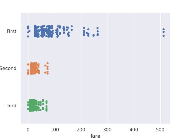
We are using the parameter jitter for making the strip plot in this example. We have styled the plot by defining darkgrid in the set function. After that, we added the data sample titanic in the load_dataset and called this seaborn laod_dataset in the variable titanic. Then, we have a strip plot where the fare and class columns are assigned to the parameters x and y from the titanic dataset. It compared the plot with this two-column. Then, we passed an option jitter and assigned it a value of 0.15. The code of the seaborn strip plot is affixed here.
The following strip plot representation with the jitter option.
Example 4
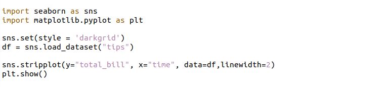
There, we have an option linewidth which we are using in the strip plot to see the working of it. Initially, we have set the background of the plot as darkgrid. Then, we have built-in dataset tips given in a seaborn. The strip plot is called and passed with the parameter for the x and y axes along with the linewidth parameter. The code of the seaborn strip plot is affixed here.
The above seaborn script outputs the following strip plot visualization.
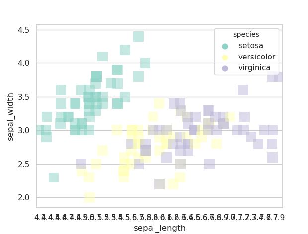
Example 5
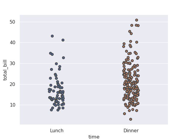
The example uses huge points and a variety of aesthetics With the help of the marker and the alpha parameter. We have utilized alpha to control the data point’s transparency, and we have modified the data point using a marker for the marker. These additional parameters are applied on the dataset iris, which we have recorded with the load_dataset command.
Then, we have a strip plot to which, with the x and y parameters, we have set the hue, palette, size, marker as r, and alpha option value as 0.15. The code of the seaborn strip plot is affixed here.
The output of the strip plot is rendered as follows:
Conclusion
There we have ended our strip plot article. The strip plot is completely self-contained. We have a brief overview of the strip plot with the seaborn module. The syntax is also clearly explained along with each parameter. To help you understand, we have shown you how to use this approach using a very easy example.