The Rolling correlation is a way of measuring the relationship between two-time series through a moving time window. This states how the correlation changes over time and detects any unusual events that affect the correlation. The rolling correlation is used to see how the sales of two products are related in different months or seasons. To determine the rolling correlation the “Rolling.corr()” method of the Pandas package is utilized in Python.
This blog offered a precise guide on determining the rolling correlation in Pandas utilizing below content:
- How to Determine the Pandas Rolling Correlation in Python?
- Determining the Rolling Correlation of DataFrame Columns
- Determining the Rolling Correlation of More Than Two DataFrame Columns
- Visualizing the Rolling Correlation of DataFrame Columns
How to Determine the Pandas Rolling Correlation in Python?
In Python, the “Rolling.corr()” method is used to determine the rolling correlation of a Pandas Series or DataFrame.
Syntax
Parameters
In this syntax:
- The “other” parameter is an optional parameter that represents another Series or DataFrame to compute the correlation with.
- The “pairwise” parameter is a Boolean value that specifies how to handle the case when both self and other are DataFrames.
- The “ddof” parameter represents the delta degrees of freedom.
- The “numeric_only” parameter specifies whether to include only integer, float, or Boolean columns.
Return Value
Series or DataFrame
Example 1: Determining the Rolling Correlation of DataFrame Columns
This example code determines the rolling correlation of two DataFrame columns:
df = pandas.DataFrame({'Months': [1, 2, 3, 4, 5, 6, 7, 8, 9, 10],
'Product_x': [23, 25, 26, 25, 27, 30, 32, 34, 35, 36],
'Product_y': [32, 34, 33, 37, 36, 36, 37, 40, 43, 42]})
print(df, '\n')
df['Correlation'] = df['Product_x'].rolling(4).corr(df['Product_y'])
print(df)
In the above code:
- We imported the “Pandas” module and constructed the DataFrame.
- After that, the “df.rolling.corr()” method is used to accept the window size “4” to determine the correlation between column “Prodcut_x” and “Product_y”. It means that for each row, it computes the correlation coefficient of the previous “4” rows of columns “Product_x” and “Product_y”.
Output
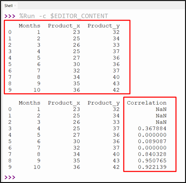
The rolling correlation between the two columns has been calculated successfully.
Example 2: Determining the Rolling Correlation of More Than Two DataFrame Columns
We can also determine the rolling correlation of more than two DataFrame columns in Python:
df = pandas.DataFrame({'Months': [1, 2, 3, 4, 5, 6, 7, 8, 9, 10],
'Product_x': [23, 25, 26, 25, 27, 30, 32, 34, 35, 36],
'Product_y': [32, 34, 33, 37, 36, 36, 37, 40, 43, 42],
'Product_z': [42, 44, 43, 47, 46, 46, 47, 50, 53, 52]})
print(df, '\n')
df['A_B_corr'] = df['Product_x'].rolling(4).corr(other=df['Product_y'])
df['A_C_corr'] = df['Product_x'].rolling(4).corr(other=df['Product_z'])
print(df)
Here:
- We initially imported the “pandas” module and constructed the DataFrame.
- Next, the “df.rolling.corr()” method is used multiple times to determine the rolling correlation of the “Product_x” column with “Product_y” and “Product_z” columns. This method takes the integer value “4” which specifies the window width.
- Lastly, the DataFrame with rolling correlation is displayed to output.
Output

The rolling correlation between multiple DataFrame columns has been shown successfully.
Example 3: Visualizing the Rolling Correlation of DataFrame Columns
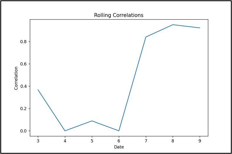
We can also visualize the rolling correlation of DataFrame columns using the “matplotlib.pyplot” module. In the below code, the “plot()”, “set_xlabel()” and “set_ylabel()” methods are used to plot the rolling correlation of DataFrame columns:
import pandas
df = pandas.DataFrame({'Months': [1, 2, 3, 4, 5, 6, 7, 8, 9, 10],
'Product_x': [23, 25, 26, 25, 27, 30, 32, 34, 35, 36],
'Product_y': [32, 34, 33, 37, 36, 36, 37, 40, 43, 42]})
print(df, '\n')
df1 = df['Product_x'].rolling(4).corr(df['Product_y'])
print(df1)
fig, ax = plt.subplots(figsize=(10, 5))
df1.plot(ax=ax)
ax.set_xlabel('Date')
ax.set_ylabel('Correlation')
ax.set_title('Rolling Correlations')
plt.show()
The visualization of the rolling correlation has been displayed successfully:
Conclusion
The “DataFrame.Rolling.corr()” method of the Pandas module is utilized to determine the rolling correlation of the Pandas Series or DataFrame. We can also employ this method to compute the rolling correlation of more than two columns. To visualize the rolling correlation the “matplotlib” module is used in Python. This write-up illustrates Pandas rolling correlation.