In this guide, we will see how to return the percentage change between the current and prior elements in Series and DataFrame. Also, for different hours frequency, this percentage is calculated.
Mathematically, Current element => (Current element – Previous element) / Previous element.
Pandas Pct_Change()
The pandas.DataFrame.pct_change() is used to compute the percentage change from the previous row. We can handle the period and fill the missing values by passing some parameters. Let’s see the parameters after the syntax.
Syntax:
Let’s see the syntax of the pct_change() function for the Pandas DataFrame:
- periods: (by default = 1) This parameter is used to shift the forming percent change. It takes an integer. For example: if periods = 2, it calculates the percent change prior to the second element from the current element.
- fill_method: (by default – “pad”) This parameter handles the missing values (NAs) before computing the percent changes. The {“backfill”, “bfill”, “ffill”, “bfill”, “None”} are the techniques that fills NA’s. Like how “ffill” fetches and places NA with the previous non-NA value, “bfill” fetches and places NA with the next non-NA value, pad places NA with 0.
- limit: (by default = None) It takes an integer that specifies the number of consecutive NA to fill before stopping to fill.
- freq: When we work with the datetime data that is related to the Time Series, this parameter can be used which is used to calculate the percent change based on the provided frequency like H – Hours, D – Day, etc.
- axis: (by default = 0) Calculate the percent change across the columns. To calculate across rows, set the axis to 1.
The pandas.DataFrame.pct_change() is used to compute the percentage change from the previous value that is present in the series. The syntax is the same as DataFrame. But it does not take axis = 1 since the columns do not exist in the Series as it is a one-dimensional data structure.
Syntax:
Let’s see the syntax of the pct_change() function for the Pandas Series:
Default Parameters
In this scenario, we pass the parameters with default values to the pct_change() function.
Example 1: Series
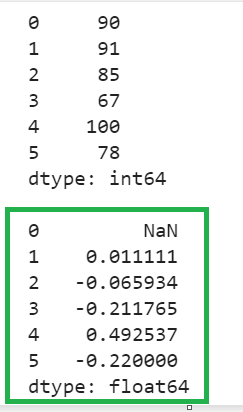
We create a “stocks” Series with six values and compute the percentage change between the current and a previous element. The default parameters are passed to this function.
# Create Series - 'stocks' with 6 values
stocks = pandas.Series([90, 91, 85,67,100,78])
print(stocks,"\n")
# With default parameters
print(stocks.pct_change(periods=1, fill_method='pad', limit=None, freq=None,axis=0))
Output:
Explanation:
- The percent change for the first element is NaN since it has no preb=vious value to compute the PCT.
- 91 => previous value is 90. So, the percent change is => (91-90)/90 => 0.011111.
- 85 => previous value is 91. So, the percent change is => (85-91)/91 => -0.065934.
Similarly, the function is calculated for the remaining two rows.
Example 2: DataFrame
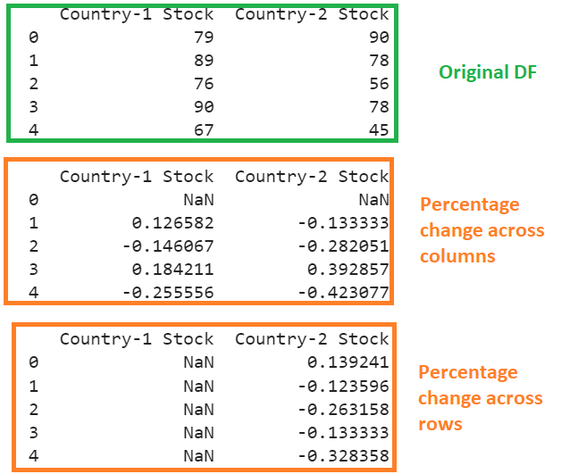
Now, we create the “stocks” DataFrame with two columns and five records.
- Compute the percentage change across the columns.
- Compute the percentage change across the rows.
# Create DataFrame - stocks with two columns
stocks = pandas.DataFrame({'Country-1 Stock':[79,89,76,90,67],'Country-2 Stock':[90,78,56,78,45]})
print(stocks,"\n")
# Percentage change across columns
print(stocks.pct_change(axis=0),"\n")
# Percentage change across rows
print(stocks.pct_change(axis=1),"\n")
Output:
Explanation:
- The first output is the original DataFrame.
- Second Output: For each column, the percent change is computed as (row [i] – row [i-1])/ row [i-1]. For example, consider the value that is present at the row index 1 => (89 – 79) /79 => 0.126582. Similarly, it is calculated for all the values.
- Last Output: The percent change is computed as (existing_col[element_pos] – previous_col[element_pos])/previous_col[element_pos]. For example, consider the first value of the first column (Country-1 Stock) – 79. The previous column does not exist. So, NaN is the pct value for 79. Also consider the first element value of the second column (Country-2 stock) – 90. The previous column is “Country-2 stock” and the first element in this column is 79. So, (90-79)/79 => 0.139241.
Periods Parameter
Let’s pass the “periods” parameter by setting different values to it.
Example 1: Series
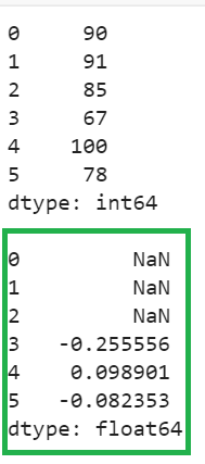
Utilize the same Series that is created in the first scenario under Example 1 and pass the “periods” parameter by setting it to 3.
# Create Series - 'stocks' with 6 values
stocks = pandas.Series([90, 91, 85,67,100,78])
print(stocks,"\n")
# With periods parameter
print(stocks.pct_change(periods=3))
Output:
Explanation:
- The percent change for the first three elements is NaN since the first three previous values do not exist for these elements.
- For the value of 67, the third previous value is 90. So, (67-90)/90 => -0.255556.
- For the value of 100, the third previous value is 91. So, (100-91)/91 => 0.098901.
- For the value of 78, the third previous value is 85. So, (78-85)/85 => -0.082353.
Example 2: DataFrame
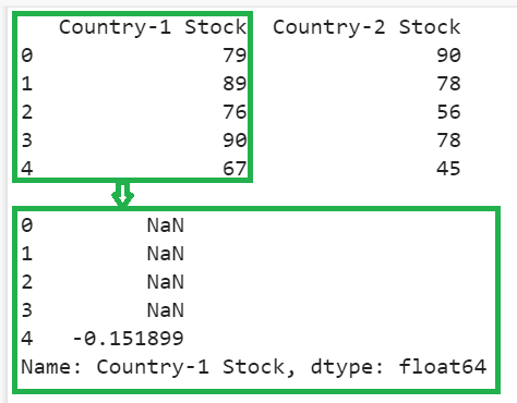
Utilize the same Data Frame that is created in the first scenario under Example 2. Calculate the percentage change for the values under the “Country-1 Stock” column by setting the periods to 4.
# Create DataFrame - stocks with two columns
stocks = pandas.DataFrame({'Country-1 Stock':[79,89,76,90,67],'Country-2 Stock':[90,78,56,78,45]})
print(stocks,"\n")
# With periods parameter
print(stocks['Country-1 Stock'].pct_change(periods=4),"\n")
Output:
Explanation:
- The percent change for the first four elements is NaN since the first four previous values do not exist for these elements.
- The last element is 67. The fourth previous element is 79 => (67-79)/79 => -0.151899.
Fill_Method Parameter
In this scenario, we specify the fill_method parameter with ffill and bfill to the pct_change() function. Both the examples that are discussed in this scenario are on the Series data structure.
Example 1: Fill_Method: Ffill (Forward Fill)
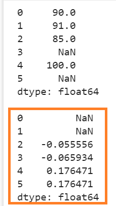
Create the “stocks” Series with six values (two missing exists). Compute the percentage change by passing the fill_method parameter as ffill. Here, before computing the percentage change for a null value, it considers the previous not-null value instead of null and then compute the percent change.
# Create Series - 'stocks' with 6 values
stocks = pandas.Series([90, 91, 85,None,100,None])
print(stocks,"\n")
# With fill_method parameter along with periods
print(stocks.pct_change(periods=2, fill_method='ffill'))
Output:
Explanation:
- The null value exists in the fourth position. The first not-null value is 85. So, 85 replaces NaN. The “periods” parameter is set to 2. So, (85-90)/90 => -0.55556.
- The null value exists in the sixth position also. The first not-null value is 100. So, 100 replaces NaN. The “periods” parameter is set to 2. So, (100-85)/85 => 0.176471.
- The other not null values are computed based on the existing values.
Example 2: Fill_Method: Bfill (Backward Fill)
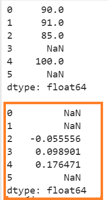
Compute the percentage change by passing the fill_method parameter as bfill.
Here, before computing the percentage change for a null value, it considers the next not-null value instead of null and then compute the percent change.
# Create Series - 'stocks' with 6 values
stocks = pandas.Series([90, 91, 85,None,100,None])
print(stocks,"\n")
# With fill_method parameter
print(stocks.pct_change(periods=2, fill_method='bfill'))
Output:
Explanation:
- The null value exists in the fourth position. The next not-null value is 100. So, 100 replaces NaN. The “periods” parameter is set to 2. So, (100-91)/91 => 0.098901.
- The null value exists in the sixth position also. The next not-null value does not exist. So, the result is NaN.
- The other not null values are computed based on the existing values.
Freq Parameter
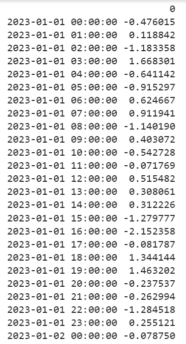
In this scenario, we apply the function on the DateTime data by specifying the “freq” parameter. First, we create a DataFrame with the DataTime as the index. The date starts from 1st January 2023 – 12: 00 AM and ends on 2nd January 2023 – 12: 00 AM.
DataFrame:
import numpy
daterange =pandas.date_range(start ='1-1-2023',end ='1-2-2023', freq ='H')
dataframe = pandas.DataFrame(numpy.random.randn(len(daterange)),index=daterange)
print(dataframe)
Output:
Example 1:
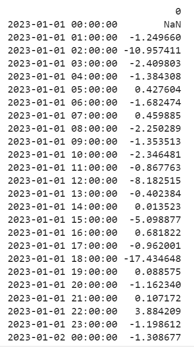
Compute the percentage change for every one hour. Here, “H” is set as frequency.
print(dataframe.pct_change(freq='H'))
Output:
Explanation:
The existing data represents the one hour frequency. We check for the second element which is 0.118842.
=> (0.118842 + 0.476015)/-0.476015
=> 0.594857/-0.476015
=> -1.249660
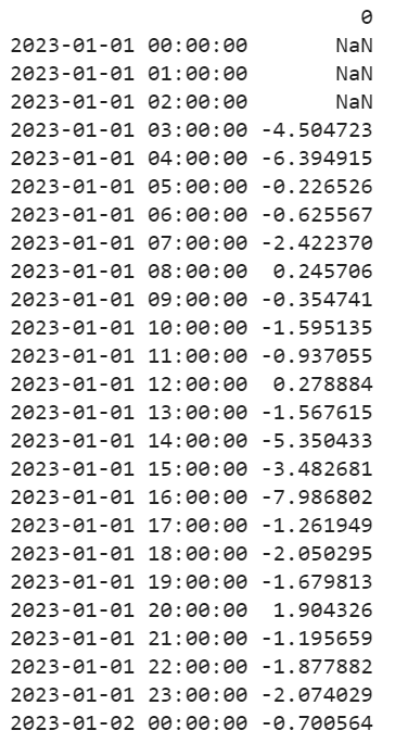
Example 2:
Compute the percentage change for every three hours. Here, “3H” is set as frequency.
print(dataframe.pct_change(freq='3H'))
Output:
Explanation:
The existing data represents the three hour frequency. We check for the fourth element which is 1.668301.
=> (-2.409803 + 0.476015)/-0.476015
=> 2.144316/-0.476015
=> -4.50
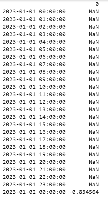
Example 3:
Compute the percentage change for every one day. Here, “D” is set as frequency.
print(dataframe.pct_change(freq='D'))
Output:
Explanation:
All are NaN except the last value.
=> ( 0.476015 - 0.078750)/-0.476015
=> 0.398515/-0.476015
=> -0.83
Conclusion
We learned how to calculate the percentage change between the current and prior elements in the Series and DataFrame using the pct_change() function. All the parameters are explained as different examples to understand the concept better. Lastly, we learned how to calculate the percentage change based on the DateTime parameters like hours and day.

