- How to Calculate Pandas Exponential Moving Average in Python?
- Determine Exponential Weighted Moving Average
- Visualize Exponential Weighted Moving Average
- Bonus: How to Calculate a simple moving average in Python?
How to Calculate Pandas Exponential Moving Average in Python?
The “DataFrame.ewm()” is a function in pandas that is utilized to perform exponentially weighted moving average (EWMA) calculations on a DataFrame. The exponentially weighted calculations assign more weightage to recent/new observations than older/last ones.
Syntax
Parameters
In the above syntax:
- The “com” parameter and the “span” parameter indicate the reduction in the center of mass and the span for the weighting function.
- The “halflife” and “alpha” parameters specify the half-life and the smoothing factor for the weighting function.
- The “min_periods” indicates the minimum number of observations needed to have a correct output/result.
- The “adjust” parameter indicates whether to divide by the decaying adjustment factor in the beginning periods.
- The “ignore_na” specifies whether to ignore missing values when calculating weights.
For other syntax functionality, you can check the official documentation.
Return Value
The return value of the “DataFrame.ewm()” function is a new DataFrame that contains the EWMA of the original DataFrame.
Example 1: Determine Exponential Weighted Moving Average
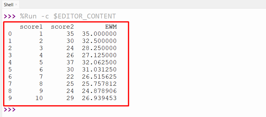
The following code is used to determine an exponentially weighted moving average for a specified number of previous/last periods. To determine the EWMA for three previous periods, the “span=3” is passed to the “ewm()” function. The span parameter specifies the number of periods to use for the EWMA. In this case, the adjust parameter is set to False, which means that the weights are not adjusted.
data1 = pandas.DataFrame({'score1': [1, 2, 3, 4, 5, 6, 7, 8, 9, 10],
'score2': [35, 30, 24, 26, 37, 30, 22, 25, 24, 29]})
data1['EWM'] = data1['score2'].ewm(span=3, adjust=False).mean()
print(data1)
The below output of the ewm() function is a new DataFrame that contains the EWMA of the original DataFrame:
Example 2: Visualize Exponential Weighted Moving Average
The “matplotlib” library can also be utilized to visualize the DataFrame column “score2” compared to the 3-day exponentially weighted moving average:
import matplotlib.pyplot as plt
data1 = pandas.DataFrame({'score1': [10, 20, 3, 40, 5, 60, 7, 80, 9, 10],
'score2': [35, 30, 24, 26, 27, 30, 22, 25, 24, 29]})
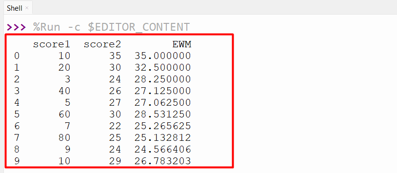
data1['EWM'] = data1['score2'].ewm(span=3, adjust=False).mean()
print(data1)
plt.plot(data1['score2'], label='score2')
plt.plot(data1['EWM'], label='EWM')
plt.legend(loc=2)
plt.show()
The below output shows the DataFrame columns containing the exponential weighted average with a span of three days:
The below graph visualizes the column “score2” compared to the EWMA:

Bonus: How to Calculate a simple moving average in Python?
The “pandas.rolling()” function is used to determine the simple moving average in Python. Here is an example code that determines the simple moving average:
import matplotlib.pyplot as plt
data1 = pandas.DataFrame({'score1': [10, 20, 3, 40, 5, 60, 7, 80, 9, 10],
'score2': [35, 30, 24, 26, 27, 30, 22, 25, 24, 29]})
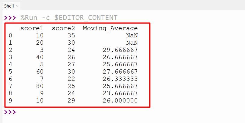
data1 = data1.assign(Moving_Average = data1['score2'].rolling(3).mean())
print(data1)
The following output displays the simple moving average:
Conclusion
The “DataFrame.ewm()” function of the “pandas” library is used to execute exponentially weighted moving average computation on a DataFrame. In this exponentially weighted calculation, the “ewm()” function assigns more weight to recent/new observations than older ones. This write-up delivered a precise tutorial on retrieving the exponential moving average using several examples.