In this tutorial, we are going to see the numpy(polyfit) regression model.
The function numpy.polyfit () finds the best fit line by minimizing the sum of squared error. This method accepts three parameters:
- x – input data
- y- output data
- Polynomial degree value (integer)
So, let’s start the step-by-step process to use the method polyfit.
Step 1: Import all the required library and packages to run this program.
Line 91: We import the NumPy and matplotlib library. The polyfit automatically comes under the NumPy, so no need to import. The matplotlib is used to plot the data and matplotlib inline is used to draw the graph inside of the jupyter notebook itself.
import matplotlib.pyplot as plt
%matplotlib inline
Step 2: Now, our next step is to create dataset (x and y).
Line 83: We randomly generate the x and y data.
y= [8, 8, 9, 72, 22, 51, 85, 4, 75, 48, 72, 1, 62, 37, 75, 42, 75, 47, 57, 95]
Step 3: We are just going to plot the feature (x) and target (y) on the graph as shown below:
Step 4: In this step, we are going to fit the line on the data x and y.
This step is very easy because we are going to use the concept of the polyfit method. The polyfit method directly comes with the Numpy as shown above. This method accepts three parameters:
- x – input data
- y- output data
- Polynomial degree value (integer)
In this program, we are using the polynomial degree value 1, which says that it is a first-degree polynomial. But we can also use it for second and third-degree polynomial.
When we press the enter, the polyfit calculates the linear regression model and store to the right-hand side variable model.
Logic Behind the Fitting Line
So, we can see that just hitting the enter key and we got out linear regression model. So now we are thinking that, what actually works behind of this method and how they fitting the line.
The method which works behind of the polyfit method is called ordinary least square method. Some people called this with the short name OLS. It is commonly used by the users to fit the line. The reason behind is it’s very easy to use and also gives accuracy above 90%.
Let’s see how OLS perform:
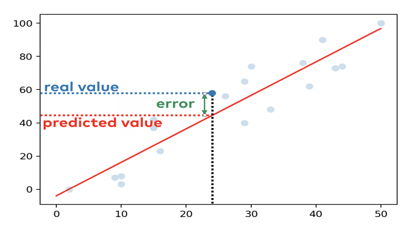
First, we need to know about error. The error calculates through the difference between the x and y data.
For example, we fit a line on the regression model which looks like below:
The blue dots are the data points and the red line which we fit on the data points using the polyfit method.
Let’s assume x = 24 and y = 58
When we fit the line, the line calculates the value of y = 44.3. The difference between the actual and calculated value is the error for the specific data point.
So, the OLS (ordinary least square) method calculates the fit using the below steps:
1. Calculates the error between the fitted model and the data points.
2. Then we square each of the data points error.
3. Sum all the square data points error.
4. Finally, identify the line where this sum of the squared error is minimum.
So, the polyfit uses the above methods to fit the line.
Step 5: Model
We have done our machine learning coding part. Now, we can check the values of x and y which are stored in the model variables. To check the x and y value, we have to print the model as shown below:
Finally, we got an outline equation:
y = 1.75505212 * x – 1.27719099
By using this linear equation, we can get the value of y.
The above linear equation can also be solved using the ploy1d() method like below:
x_value = 20
predict(x_value)
We got the result 33.82385131766588.
We also got the same result from the manual calculation:
y = 1.75505212 * 20 – 1.27719099
y = 33.82385131766588
So, both the above results show that our model fits the line correctly.
Step 6: Accuracy of the model
We can also check the accuracy of the model, either it gives correct results or not. The accuracy of the model can be calculated from the R-squared (R2). The value of the R-squared (R2) is between 0 and 1. The result close to 1 will show that model accuracy is high. So, let’s check for the above model accuracy. We will import another library, sklearn, as shown below:
r2_score(y, predict(x))
The result shows that it is close to 1, so its accuracy is high.
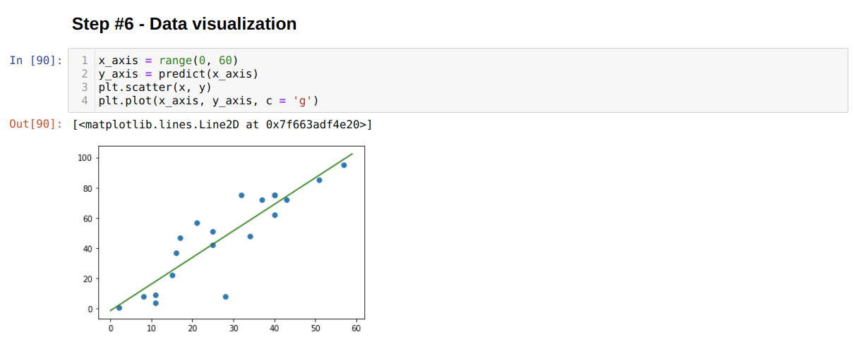
Step 7: Plotting the model
The plotting is the method to see the model fitted line on the data points visually. It gives clear image of the model.
y_axis = predict(x_axis)
plt.scatter(x, y)
plt.plot(x_axis, y_axis, c = 'g')
A quick explanation for the above plot method is given below:
Line 1: It is the range which we want to display on the plot. In our code, we are using the range value from 0 to 60.
Line 2: All the range values from 0 to 60 will be calculated.
Line 3: We pass those x and y original datasets into the scatter method.
Line 4: We finally plot our graph, and the green line is the fit line as shown in the above graph.
Conclusion
In this article, we have learned the linear regression model which is the start of the journey of machine learning. There is a number of regression models that are explained in another article. Here, we have a clean dataset because that was a dummy, but in real-life projects, you might get a dirty dataset and you have to do feature engineering on that to clean the dataset to use in the model. If you do not fully understand this tutorial, even that helps you to learn another regression model easily.
The line regression model is the most common algorithm used by data science. You must have ideas about the regression model if you want to have your career in this field. So, keep in touch and soon we will be back with a new data science article.
The code for this article is available at the Github link:
https://github.com/shekharpandey89/Linear-Regression-in-Python—using-numpy-polyfit


