Curve fitting is the way of fitting the function in data points. This method is used to plot the best-fit line in MATLAB. This is a complicated method but MATLAB makes it easy by offering various curve fitting functions. One such function is the polyfit() which can plot a best-fit line in MATLAB.
This guide is going to explain how to use the polyfit() function in MATLAB using some examples.
What is Curve Fitting?
Curve fitting is a method of finding the mathematical function that best fits the set of data points; it will help you in finding a function that minimizes the error between the function and the data points. There are several curve fitting methods, each having its own advantages and disadvantages, some of the most common methods are:
- Simple Linear Regression: A common type of regression utilized for finding a straight line that best fits the data points.
- Polynomial Regression: This type of regression involves identifying the polynomial function that best fits the data points.
- Non-Linear Regression: This type of regression is used for finding the nonlinear function that best fits the data points.
How to Use polyfit() Function in MATLAB?
MATLAB facilitates us with a built-in polyfit() function to plot the best-fit line. This function is used for data approximation by fitting the curve in the given data points. If we have n data points, it becomes possible to write the polynomial having degree less than n-1 that may or may not pass through all data points, using the polyfit() function.
Syntax
The polyfit() function follows a simple syntax in MATLAB that is given below:
[p,S] = polyfit(x,y,n)
[p,S,mu] = polyfit(x,y,n)
Here,
The function p = polyfit(x,y,n) provides the coefficients for the polynomial p(x) having degree n that yields the best-fit line using the least square method for the data in y. The p has length n+1, and the p’s coefficients have powers in descending order.
The function [p, S] = polyfit(x,y,n) gives the structure S, which can be used in the polyval() function as an argument for getting error estimates.
The function [p, S, mu] = polyfit(x,y,n) returns a mu vector with two elements having values for centering and scaling. The mu(1) is equivalent to mean(x), whereas mu(2) is equal to std(x). Utilizing these settings, polyfit() scales x to have a unit standard deviation where it centers x at zero.
Examples
Follow the given examples to understand the working of MATLAB’s polyfit() function.
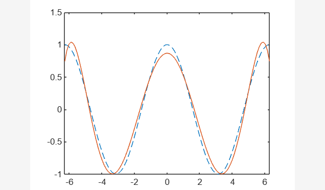
Example 1: How to Fit Polynomial to Trigonometric Function Using the polyfit() Function?
The given example creates a linearly spaced vector along the cosine curve having 100 elements. After that, it uses the polyfit() function to fit the 6th-degree polynomial in the given function. Finally, it estimates the polynomial on the finer grid and plots the results.
y = cos(x);
p = polyfit(x,y,6);
x1 = linspace(-2*pi,2*pi);
y1 = polyval(p,x1);
figure
plot(x,y,'--')
hold on
plot(x1,y1)
hold off
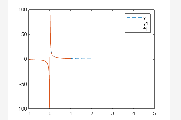
Example 2: How to Fit a Polynomial to the Set of Points Using the polyfit() Function?
This example creates a linearly spaced vector having 100 elements and evaluates the given function on each element of x. After that, it uses the polyfit() function to fit the 8th-degree polynomial in the given function, then finally estimates the polynomial on the finer grid and plots the results.
y = 1./x;
p = polyfit(x,y,8);
x1 = linspace(-1,1);
y1 = 1./x1;
f1 = polyval(p,x1);
figure
plot(x,y,'--')
hold on
plot(x1,y1)
plot(x1,f1,'r--')
legend('y','y1','f1')
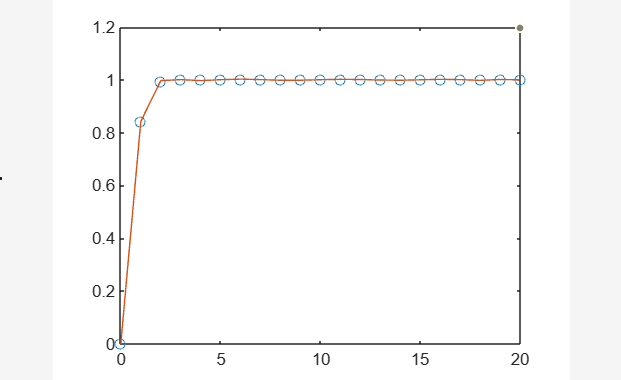
Example 3: How to Fit Polynomial to Error Function Using the polyfit() Function?
The given MATLAB code first creates a vector x with 21 equally spaced elements in the interval [0, 20]. Then it finds values of y corresponding to all x’s using the error function erf(x). After that, it uses the polyfit() function to fit the 10th-degree polynomial in the given data points. At last, it plots the polynomial evaluation results with a finer grid.
y = erf(x);
p = polyfit(x,y,10);
f = polyval(p,x);
plot(x,y,'o',x,f,'-')
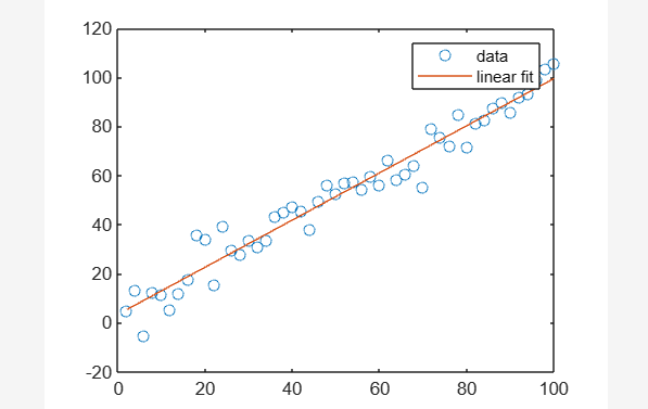
Example 4: How to Perform Simple Linear Regression Using the polyfit() Function?
The given example defines a vector x with 50 evenly spaced elements lying in the interval [2, 100]. Then it finds values of y corresponding to all x’s. After that, it uses the polyfit() function for fitting the 1st-degree polynomial in the given data points (x,y) and evaluates the fitted polynomial p at x. At last, it plots the obtained linear regression model with the data points.
y = x + 5*randn(1,50);
p = polyfit(x,y,1);
f = polyval(p,x);
plot(x,y,'o',x,f,'-')
legend('data','linear fit')
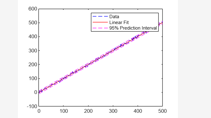
Example 5: How to Perform Linear Regression With Error Estimate Using the polyfit() Function?
The given MATLAB code first creates a vector x with 500 equally spaced elements in the interval [1, 500]. Then it finds values of y corresponding to all x’s. After that, it uses the polyfit() function for fitting the 1st-degree polynomial in the given data points (x,y) and evaluates the fitted polynomial p at x. At last, it plots the original linear regression and 95% precision interval with the data points.
y = x + 5*randn(1,500);
[p,S] = polyfit(x,y,1);
[y_fit,delta] = polyval(p,x,S);
plot(x,y,'--b')
hold on
plot(x,y_fit,'r-')
plot(x,y_fit+2*delta,'m--',x,y_fit-2*delta,'m--')
legend('Data','Linear Fit','95% Prediction Interval')
Conclusion
MATLAB includes a built-in polyfit() function to plot the best-fit line. This function allows us to approximate the data by fitting the curve in the given data points. If we have n data points, the polynomial having degree less than n-1 can give the best approximation for the given n data points. This guide provided information about curve fitting and taught us how to use the polyfit() function in MATLAB.