The initial value problems (IVP) play an important role in solving any physical phenomenon used in engineering applications. These problems can be solved using analytical and numerical methods. There are limited methods for solving the initial value problems analytically. So, most of the time we adopt numerical methods for solving them.
Solving an initial value problem numerically is not an easy task but MATLAB makes it easy by introducing built-in functions like ode23, ode45, and many others.
This blog is going to explore how to solve an initial value problem in MATLAB using the ode45() function.
What is an Initial Value Problem?
An initial value problem includes a differential equation with one or more initial conditions based on the order of the differential equation. The initial value problem has the standard form that is given below:

Here y behaves like a dependent variable while x behaves like an independent variable.
How to Solve an IVP Using the Function ode45()?
An initial value problem having initial conditions can be solved analytically and numerically. However, to get an accurate solution, we use numerical methods. MATLAB supports some built-in functions for numerically solving the initial value problems. One such function is ode45(). This function works the same as the Runge-Kutta method. The Runge-Kutta or RK method is a numerical method used for solving initial value problems and is known for its accuracy and stability.
Syntax
The ode45() function uses a simple syntax in MATLAB.
Here:
The function [t,y] = ode45(odefun,tspan,y0) calculates and returns the numerical solutions of the given initial value problem where tspan integrates the given function from t0 to tf on the given initial condition y0.
Examples
Consider some examples to learn how to use the ode45() function to solve an initial value problem in MATLAB.
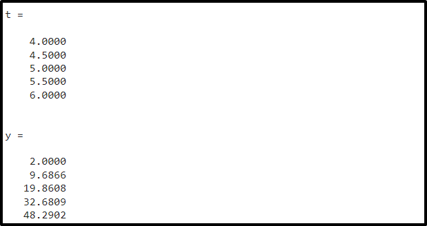
Example 1: How to Solve 1st Order ODE Using Initial Condition in MATLAB Using ode45() Function?
In this example, we first create a user-defined function ivp1.m that includes the 1st ODE.
dydt=(3*t^2+2*y)/t;
After that, we use the ode45() function to evaluate the given IVP on the specified initial conditions.
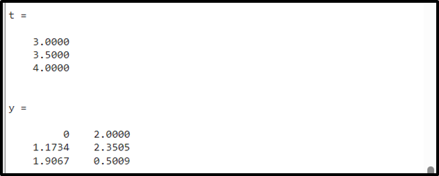
Example 2: How to Solve 2nd Order ODE Using Initial Condition in MATLAB Using ode45() Function?
This example first creates a user-defined function ivp2.m that includes the 2nd-order ODE.
dydt = [y(2); (1-y(1)^2)*y(2)-y(1)];
After that, it uses the ode45() function to evaluate the given IVP on the given initial conditions.
Conclusion
The initial value problems are widely used for solving physical phenomena of engineering applications. These problems can be computed using numerical as well as analytical techniques. The numerical methods obtain more accurate solutions than the analytical methods. MATLAB facilitates us with built-in functions to solve initial value problems numerically. One such function is the ode45() function which uses the RK method to solve these problems. This tutorial has provided the approach to solving initial value problems using the ode45() function in MATLAB. The examples explained in this tutorial will assist you in learning the workings of this function in MATLAB.