The “seaborn” is one of the most popular libraries for data visualization in Python, and it provides a variety of plotting functions that can create interactive and informative plots. Saving seaborn plots in various formats is helpful to share the plots with others easily, regardless of the software or platform, and it also saves time and effort.
In this article, we will explore the approaches to save the seaborn plots in different file formats and customize the plot settings for optimal output.
Note: Before creating “seaborn” plots, we need to set up the library in our Python environment. The “seaborn” can be installed using “pip”, which is the most common way of installing Python packages via the following command:
How to Create a Plot With Seaborn in Python?
To create a plot with seaborn, various functions are used in Python. In the below example code, the “seaborn.scatterplot()” function is used to create the scatter plot of the provided dataset.
Example
Let’s overview the following example code:
import matplotlib.pyplot as plt
import pandas
df = pandas.DataFrame({"Day 1": [17,11,15,16,23,10,15,18],
"Day 2" : [31,22,38,44,34,92,54,22]})
seaborn.scatterplot(data=df)
plt.show()
In the above code, the “seaborn”, “matplotlib” and “pandas” libraries are imported, respectively. After that, the “seaborn.scatterplot()” function takes the data from the created Data Frame and creates scatter plots with different semantic groupings.
Output
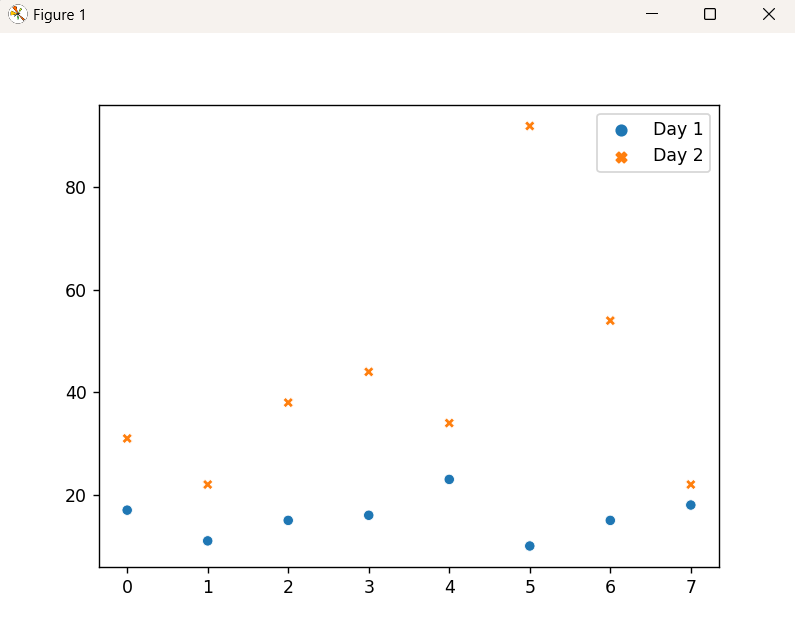
As seen, the scatter plot of the provided dataset has been created.
How to Save a Python Seaborn Plot to a File?
Once we have created a plot, we can save it to a file using the “savefig()” function from matplotlib. This function takes the filename as input and saves the plot to that file. The “seaborn” library allows you to save plots in various formats, including “png”, “jpg”, or “pdf”. Let’s explore the approaches to saving seaborn plots in different formats.
Saving “seaborn” Plots in “png” Format
The “PNG” format offers transparent backgrounds while maintaining lossless quality. To save a seaborn plot in “png” format, apply the matplotlib “savefig()” function.
Example
The following code example demonstrates how it works:
import matplotlib.pyplot as plt
import pandas
df = pandas.DataFrame({"Day 1": [17,11,15,16,23,10,15,18],
"Day 2" : [31,22,38,44,34,92,54,22]})
seaborn.scatterplot(data=df)
plt.savefig("scatter_plot.png")
In the above lines of code, the “savefig()” function saves the plot in the current directory by default with the given filename. We can also specify a different directory or file format as per the requirement.
Output
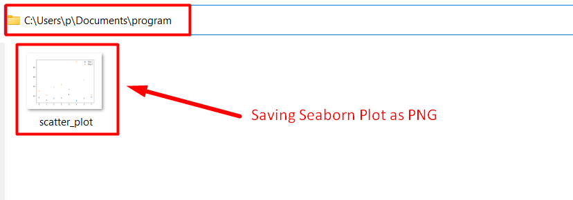
As analyzed, the seaborn plot has been saved in the “PNG” format appropriately.
Saving “seaborn” Plots in “jpg” Format
“jpg” is a lossy image format that supports a wide range of colors and can compress images to small sizes. To save a seaborn plot in this particular format, likewise, apply the matplotlib “savefig()” function.
Example
Let’s understand it by considering the following example:
import matplotlib.pyplot as plt
import pandas
df = pandas.DataFrame({"Day 1": [17,11,15,16,23,10,15,18],
"Day 2" : [31,22,38,44,34,92,54,22]})
seaborn.scatterplot(data=df)
plt.savefig("scatter_plot.jpg")
In the above code snippet, the applied “plt.savefig()” function saves the plot based on the created Data Frame by specifying the file name and the desired format i.e., “jpg”, respectively.
Output
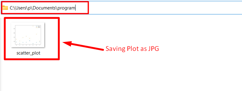
Here, the plot has been saved with the specified name and in the desired format accordingly.
Saving “seaborn” Plots in “pdf” Format
“pdf” is a vector-based image format that supports high-quality graphics and is suitable for publication. The matplotlib “savefig()” function can be applied here as well to save a seaborn plot in “pdf” format.
Example
The below-provided example saves the seaborn plot in the particular format i.e., “pdf”:
import matplotlib.pyplot as plt
import pandas
df = pandas.DataFrame({"Day 1": [17,11,15,16,23,10,15,18],
"Day 2" : [31,22,38,44,34,92,54,22]})
seaborn.scatterplot(data=df)
plt.savefig("scatter_plot.pdf")
In the above code, recall the discussed approach for creating a data frame. Now, apply the “plt.savefig()” function to save the plot in “pdf” format.
Output
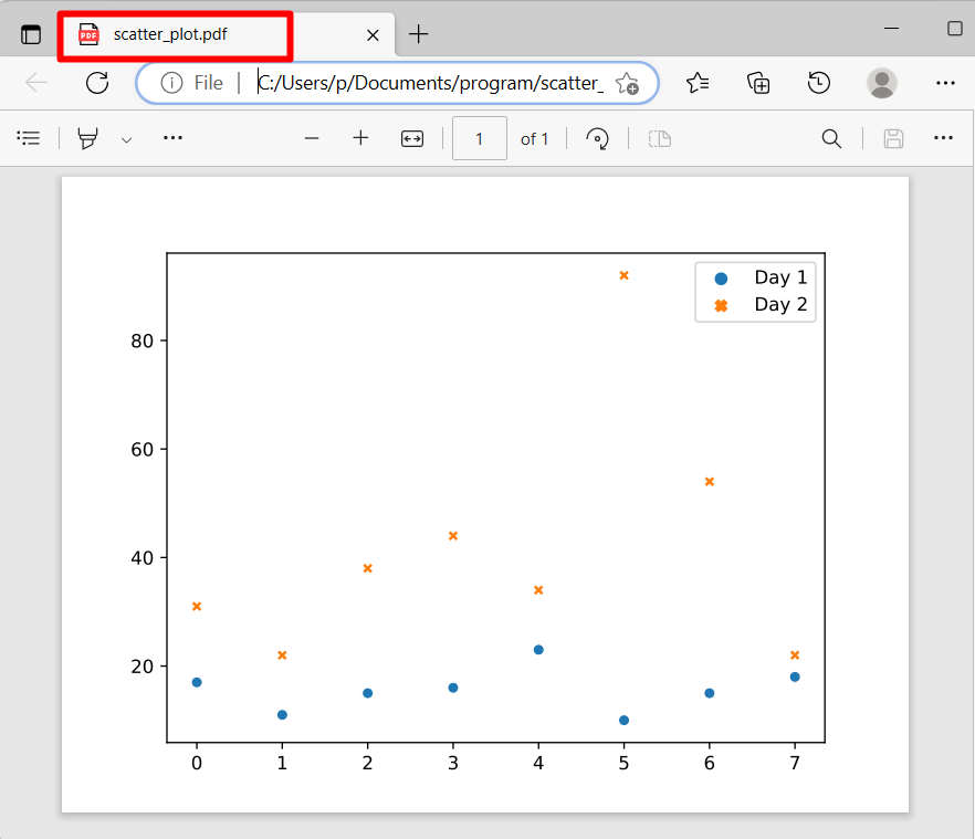
As observed, the plot has been saved as “pdf”.
How to Customize Plot Settings For Saving in Python?
The “seaborn” library allows you to customize plots by changing various aspects of the plot, such as colors, labels, titles, etc. The “seaborn” plots can be customized before saving to make the plot more informative and visually appealing.
Example
Let’s overview the below-stated code:
import matplotlib.pyplot as plt
import pandas
df = pandas.DataFrame({"Day 1": [17,11,15,16,23,10,15,18],
"Day 2" : [31,22,38,44,34,92,54,22]})
seaborn.scatterplot(data=df)
plt.title("Dataset")
plt.xlabel("Day-1")
plt.ylabel("Day-2")
plt.savefig("seaborn_plot_custom.png")
In the above code block, we added a title and labels to the plot, respectively, and saved the plot in “png” format.
Output
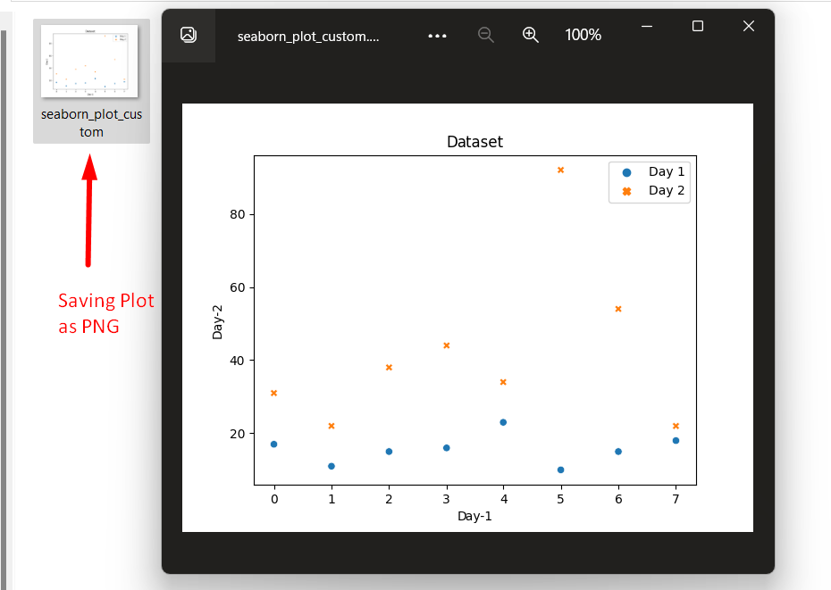
In the above outcome, it can be implied that the customized plot has been saved in the “PNG” format appropriately.
Conclusion
The matplotlib “plt.savefig()” function can be applied to save seaborn plots in various formats, including “png”, “jpg”, or “pdf”. These plots can be customized as well as per the requirement. This post presented an in-depth guide to saving seaborn plots in Python.