Plotting multiple functions in MATLAB provides a powerful tool for visualizing and comparing mathematical relationships within a single graph. Whether you’re analyzing data or exploring mathematical concepts, MATLAB offers various methods to plot multiple functions efficiently. In this article, we will explore different techniques and code examples to plot multiple functions in MATLAB, empowering you to create informative and visually appealing plots.
How To Plot Multiple Functions in MATLAB
Plotting multiple functions in MATLAB is significant as it allows for visual comparison and analysis of different mathematical relationships within a single graph, enabling insights into their behavior and interactions. Below are some common techniques to plot multiple functions in MATLAB:
Method 1: Plot Multiple Functions in MATLAB using Sequential Plotting
One straightforward approach is to plot each function sequentially using multiple plot() commands, here is an example:
% Calculate the y-values for each function
f = sin(x);
g = cos(x);
% Plot each function sequentially
plot(x, f, 'r-', 'LineWidth', 2); % Plots f(x) in red with a solid line
hold on; % Allows for overlaying subsequent plots
plot(x, g, 'b--', 'LineWidth', 2); % Plots g(x) in blue with a dashed line
hold off; % Ends the overlaying of plots
% Add labels and title
xlabel('x');
ylabel('y');
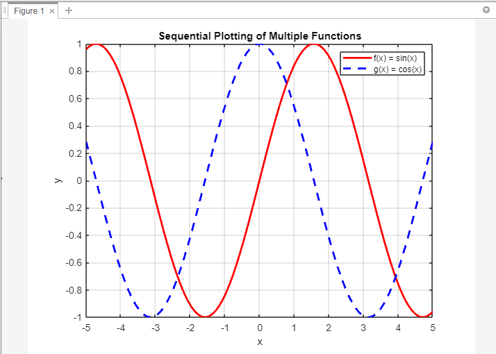
title('Sequential Plotting of Multiple Functions');
% Add a legend
legend('f(x) = sin(x)', 'g(x) = cos(x)');
% Display the grid
grid on;
The code first defines the x-values using linspace() to create a range of values from -5 to 5 with 100 points. The y-values for two functions, f(x) = sin(x) and g(x) = cos(x), are then calculated using the corresponding mathematical expressions.
Next, the functions are plotted sequentially using the plot() function. The first plot() command plots f(x) in red with a solid line, while the second plot() command plots g(x) in blue with a dashed line. The hold on and hold off commands are used to overlay subsequent plots without clearing the previous ones.
Method 2: Plot Multiple Functions in MATLAB using Vectorized Plotting
MATLAB’s vectorized operations allow plotting multiple functions using a single plot() command by combining the x-values and corresponding y-values into matrices. Here’s an example:
% Calculate the y-values for each function
f = sin(x);
g = cos(x);
% Combine x-values and y-values into matrices
xy1 = [x; f];
xy2 = [x; g];
% Plot multiple functions using vectorized plotting
plot(xy1(1,:), xy1(2,:), 'r-', 'LineWidth', 2); % Plots f(x) in red with a solid line
hold on; % Allows for overlaying subsequent plots
plot(xy2(1,:), xy2(2,:), 'b--', 'LineWidth', 2); % Plots g(x) in blue with a dashed line
hold off; % Ends the overlaying of plots
% Add labels and title
xlabel('x');
ylabel('y');
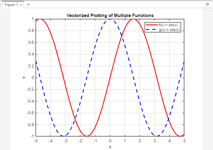
title('Vectorized Plotting of Multiple Functions');
% Add a legend
legend('f(x) = sin(x)', 'g(x) = cos(x)');
% Display the grid
grid on;
The code first defines the x-values using linspace() to create a range of values from -5 to 5 with 100 points.
Next, the y-values for two functions, f(x) = sin(x) and g(x) = cos(x), are calculated using the corresponding mathematical expressions. These x-values and y-values are then combined into matrices, xy1, and xy2, where each matrix consists of two rows: the first row represents the x-values and the second row represents the corresponding y-values.
Using vectorized plotting, the plot() function is used to plot multiple functions. The first plot() command plots f(x) by extracting the x-values from xy1(1,:) and the y-values from xy1(2,:), using a red solid line. The second plot() command plots g(x) by extracting the x-values from xy2(1,:) and the y-values from xy2(2,:), using a blue dashed line.
Method 3: Plot Multiple Functions in MATLAB using Function Handles
Another approach involves defining function handles for each function and using a loop to plot them. Here’s an example:
% Define function handles for each function
functions = {@(x) sin(x), @(x) cos(x)};
% Plot multiple functions using function handles
hold on; % Allows for overlaying subsequent plots
for i = 1:length(functions)
plot(x, functions{i}(x), 'LineWidth', 2); % Plots each function
end
hold off; % Ends the overlaying of plots
% Add labels and title
xlabel('x');
ylabel('y');
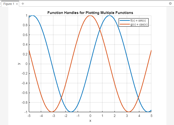
title('Function Handles for Plotting Multiple Functions');
% Add a legend
legend('f(x) = sin(x)', 'g(x) = cos(x)');
% Display the grid
grid on;
The code first defines the x-values using linspace() to create a range of values from -5 to 5 with 100 points.
Next, function handles are defined for each function using the @() notation. The functions variable is an array that holds the function handles for f(x) = sin(x) and g(x) = cos(x).
Using a loop, the code iterates through each function handle in the functions array and plots the corresponding function using the plot() function. The x-values are constant for all functions, while the y-values are obtained by evaluating each function handle with the x-values as input.
The hold on command allows for overlaying subsequent plots without clearing the previous ones. After plotting all the functions, the hold off command ends the overlaying of plots.
Conclusion
MATLAB provides several versatile approaches to plot multiple functions, offering flexibility and control over your visualizations. Whether you prefer sequential plotting, vectorized operations, or function handles, each method allows you to effectively compare and analyze mathematical relationships within a single graph.