This blog is going to explain how to plot the best-fit line in MATLAB using the polyfit() function.
How to Plot the Best Fit Line in MATLAB?
Plotting the best-fit line in MATLAB can easily be done using the built-in polyfit() function. This function is used for data approximation by fitting the curve in the given data points. The function takes multiple arguments, including the data points and the polynomial’s degree. The polyfit() function generates a coefficients vector that is used to evaluate a polynomial at any point.
If we have n data points, it becomes possible to write the polynomial having degree less than n-1 that may or may not pass through all data points, using the polyfit() function.
Syntax
The polyfit() function has several syntaxes that can be used in MATLAB for performing curve-fitting tasks:
[p,S] = polyfit(x,y,n)
[p,S,mu] = polyfit(x,y,n)
Here:
The function p = polyfit(x,y,n) provides the coefficients for the polynomial p(x) having degree n that yields the best-fit line using the least square method for the data in y. The p has length n+1, and the p’s coefficients have powers in descending order.
The function [p,S] = polyfit(x,y,n) gives the structure S, which can be used in the polyval() function as an argument for getting error estimates.
The function [p, S, mu] = polyfit(x,y,n) returns mu as a vector with two elements having values for centering and scaling. The mu(1) is equivalent to mean(x), whereas mu(2) is equal to std(x). With these options, polyfit() adjusts x so that its zero-value output has the unit standard deviation.
Examples
Follow the given examples to understand the working of the polyfit() function to plot the best-fit line in MATLAB.
Example 1: How to Plot the Best Fit Line in MATLAB Using the polyfit(x, y, n) Function?
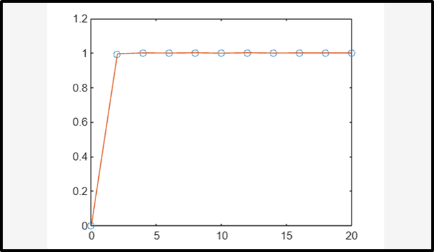
This example first creates a vector x having 11 evenly spaced elements contained by the interval [0, 20]. Then it finds values of y corresponding to all x’s using the error function erf(x). After that, it uses the polyfit() function for fitting the 9th-degree polynomial in the given data points. At last, it plots the polynomial evaluation results with a finer grid.
y = erf(x);
p = polyfit(x,y,9);
f = polyval(p,x);
plot(x,y,'o',x,f,'-')
Example 2: How to Plot the Best Fit Line in MATLAB Using the [p, S]= polyfit(x, y, n) Function?
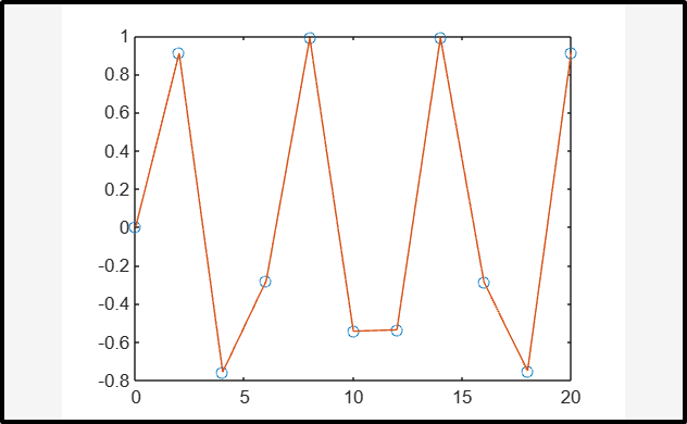
This MATLAB code first creates a vector x with 11 evenly spaced elements contained by the interval [0, 20]. Then it finds values of y corresponding to all x’s using the sin(x) function. After that, it uses the polyfit() function for fitting the 10th-degree polynomial in the given data points. At last, it plots the polynomial evaluation results with a finer grid.
y = sin(x);
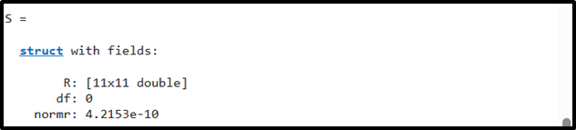
[p,S] = polyfit(x,y,10)
f = polyval(p,x);
plot(x,y,'o',x,f,'-')
Conclusion
MATLAB includes a built-in polyfit() function to plot the best-fit line. This function allows us to approximate the data by fitting the curve in the given data points. If we have n data points, the polynomial having degree less than n-1 can give the best approximation for the given n data points. This guide has provided us with information about curve fitting and helps us understand how to plot the best-fit line in MATLAB.