You will discover how to fit polynomial curves using MATLAB’s polyfit() function in this tutorial.
How to Code polyfit() in MATLAB?
To code polyfit() in MATLAB, you must first follow the below-given syntax:
[p,S] = polyfit(x,y,n)
[p,S,mu] = polyfit(x,y,n)
The above syntax can be described as:
- p = polyfit(x,y,n): provides the coefficients of the degree n polynomial p(x) that best fits the data in y in terms of least-squares. The coefficients into p are arranged in descending powers and have a length of n+1.
- [p,S] = polyfit(x,y,n): produces a structure S that can be used as an input in polyval to obtain error estimates.
- [p,S,mu] = polyfit(x,y,n): yields mu, a two-element vector with values for scaling and centering. The mu(1) is mean(x), whereas mu(2) is std(x). Using these settings, polyfit() scales x to have a unit standard deviation, where it centers x at zero.
Let’s consider some examples that demonstrate using the MATLAB polyfit() function.
Example 1
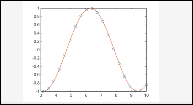
In the given example, first, we generate a vector x having 10 equally spaced elements lying in the interval (10, 20). Then we find values of y corresponding to all values of x using the trigonometric function cos(x). After that, the polyfit() function is used to fit the 6th-degree polynomial in the data points. At last, we Plot the results of the polynomial evaluation with a finer grid.
y = cos(x);
p = polyfit(x,y,6);
x_1 = linspace(10,pi);
y_1 = polyval(p,x_1);
figure
plot(x,y,'o')
hold on
plot(x_1,y_1)
hold off
Example 2
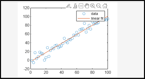
This example uses the polyfit() function to fit a simple linear regression model in a set having 2-D discrete data points. In this code, a set of data points is generated with x values ranging from 2 to 100 with a step of 2. The corresponding y values are calculated by subtracting a random noise from a linear function of x. The polyfit() function is then used to fit a linear polynomial to the data, obtaining the coefficients p. The fitted polynomial is evaluated using polyval() and plotted along with the original data points using the plot() function.
y = x - 5*randn(1,50);
p = polyfit(x,y,1);
f = polyval(p,x);
plot(x,y,'o',x,f,'-')
legend('data','linear fit')
Conclusion
The MATLAB polyfit() function is used for polynomial curve fitting. This function takes two vectors and a degree of polynomial as arguments and plots the obtained results. This tutorial provided some useful information about how to code a polyfit() function in MATLAB, with some useful examples that help beginners understand the use of this function.