Dijkstra’s Algorithm Time Complexity

Consider the following towns: A, B, C, D, E, and F connected by roads:

These towns are connected by roads (which can be assumed to be straight). The road length from town A to town B is 4 units; it is not drawn to scale. The road length from town A to town C is 5 units; it is not drawn to scale. The length from town B to town E is 11 units, not drawn to scale. The roads between other towns are similarly indicated.

The towns: A, B, C, D, E, and F are the vertices of a graph. The roads are the edges of the graph. However, this graph will be represented in a mathematical data structure, differently from its geographical layout.

Dijkstra’s algorithm can be used to find the shortest path between a source vertex (say A) and any other vertex. For further simplicity, this article will aim to look for the shortest path from A to E.

There are different paths from A to E, with different lengths, as follows:

From this listing, the shortest path is A-C-E-F, with a total length of 14 units.

The main aim of this article is to find the running time Dijkstra’s algorithm takes to obtain the shortest path from A to E. The time will not be given in seconds or minutes. It is the relative total execution time, called Time Complexity, that will be given. C++ coding is provided as well.

Graph to Use

The time complexity (relative running time) depends mainly on the type of mathematical graph used to represent the geographical layout. It also depends on the algorithm (another kind of algorithm) used to sort the neighboring vertices of each vertex in the overall algorithm (Dijkstra’s algorithm). The sorting of neighboring vertices is not addressed in this article.

The mathematical graph chosen for this article is called Adjacency Matrix. It is:

The row headers are the town names from A to F. The column headers are the same town names from A to F. Each entry is the length of a road from one town to the next. The length of a road from one town to itself is zero. The length of a road from one town to another, after skipping one or more towns, is also zero. Only direct roads are considered. Each entry is located, first by row and then by column. Again, each entry is the length of one road, without skipping a town, and not to the town itself. This matrix is a mathematical representation of the geographical network given above.

So, the matrix consists of edges, with the row and column headers of the same vertices. The matrix is the main structure needed in the program. Two other vectors (arrays) are used in this basic program.

Dijkstra’s Algorithm

Dijkstra’s algorithm looks for the shortest path between any two vertices in a graph (network). The above matrix is the graph, which corresponds to the above geographical network. For simplicity, the program in this article will look for the shortest path between a source vertex and one destination vertex. Precisely, the program will look for the shortest path from the source vertex, A, to the destination vertex, F.

The algorithm, as relevant to this task, is as follows:

– All vertices are marked as unvisited. At this point, a set of all unvisited vertices are created.

– Assign a tentative path length value to all vertices: the path length from source to the source is assigned a value of zero; the path length from source to any other vertex is assigned the one value of infinity, i.e., a value that is higher than the highest path possible, in the graph. The value of each vertex would be changed at least once, from a high value to a lower value, as the algorithm continues. Possible vertices for the complete shortest path will be focused upon, beginning from the source vertex (A). The vertex with the focus is called the current vertex. The current vertex has neighbors, better visualized from the actual network (geographical layout) above.

– There is the current vertex, and there is the visited vertex. In fact, there would be more than one visited vertex in a chain as the algorithm continues. All previous vertices considered visited are in the shortest complete path that is being developed, beginning from the source. The path length of the last visited vertex is known (should be known). A vertex is declared visited when its path length is confirmed. The visited vertex gives the least path length from the source so far, as the algorithm is in progress. The unvisited neighbors of the current vertex, except its immediate previous visited neighbor, have tentative values (path lengths from the source), some of which may still be infinity (very high value). For each unvisited neighbor and the current vertex, a new tentative path length is calculated as follows: the path length of the previously visited vertex, plus the edge length to the current vertex, plus the length of the edge from the current vertex, to the unvisited neighbor. If this result is less than what was there, as the tentative path length from the source to the unvisited neighbor of the current vertex, then this calculated value becomes the new tentative value for the neighbor of the current vertex. That is, the new tentative path value for an unvisited vertex is calculated through the current vertex from the previously visited vertex.

– There can be more than one current vertices. When all the neighbors of each current vertex have been accessed and given new appropriate tentative path lengths, the current vertex with the least path length from the source (least value) is considered visited. Since it had the least value, its least value is confirmed as the shortest part-path length so far. The previously visited vertex is removed from the unvisited vertex set. A visited vertex will never be checked again. Any visits after would have a greater path length.

– The previous two steps are repeated, in order, for any next current vertex that becomes a visited vertex. This repetition continues until the destination vertex is reached. The destination vertex can be any vertex after the source vertex. However, for simplicity, the last vertex, F of the above network, has been chosen as the destination vertex for this article.

– As the algorithm progresses, each parent (previously visited) vertex, and each child (next visited) vertex, of the shortest path should be recorded in case the shortest path, by vertices, as well as the shortest path by length, is required (asked for). When the destination vertex is reached and visited, the complete shortest path can be traced backward if the path by vertices is needed. As for the path length, it was calculated as the algorithm progressed.

Illustration Dijkstra’s Algorithm

The above road

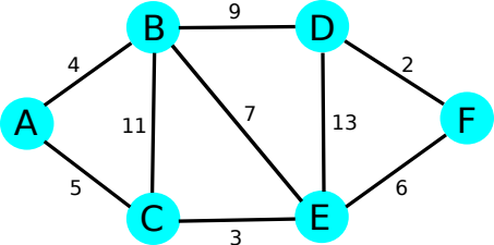
network is used to illustrate Dijkstra’s algorithm. It is re-displayed below for easy reference.

It begins at the source, “A” with a path length of zero. “A” is considered as visited and removed from the unvisited list (set). “A” is sent to a visited list in case the path by vertices will be required.

The path lengths from A to B are:

Between 4, 16, and infinity (that was there), 4 is the least. So, B is given the tentative value of 4 as path length.

The path lengths from A to C are:

Between 5, 15, and infinity (that was there), 5 is the least. So, C is given the tentative value of 5 as path length.

B and C were the unvisited neighbors of A. Currently, each has a tentative path length. Between B and C, a vertex must be chosen contribute to the final overall path. B and C also have neighbors.

The unvisited neighbors of B are D, E, and C, with tentative infinite lengths. The unvisited neighbors of C are B and E with tentative infinite lengths. A neighbor has one direct edge from the vertex in question.

The path length calculated from A to D, through B is:

The path length calculated from A to E, through B is:

The path length calculated from A to C, through B is:

Those are the path lengths through B to B’s neighbors, from the visited vertex, “A”. The tentative path lengths through C should also be determined.

The path length calculated from A to B, through C is:

The path length calculated from A to E through C is:

Those are the path lengths through C to C’s neighbors, from the visited vertex, “A”.

All the tentative calculated part-path lengths so far are:

The shortest of these part-path lengths is:

So the vertex, C, is chosen for the way forward. This is the next visited vertex. Any possible path through B is abandoned. C is then considered visited. The vertex C is removed from the unvisited list. C is sent to the visited list (to be after A).

C should have unvisited neighbors with tentative path lengths. In this case, it is B and E. B has neighbors with infinite path lengths, which are D, and E. E has neighbors with infinite path lengths, which are D and F. In order to choose the next visited node, the tentative part-path lengths from C through B and E have to be calculated. The calculations are:

The shortest for these part-paths is:

At this point, E is the way forward. This is the next visited vertex. Any possible path through D is abandoned. E is removed from the unvisited list and added to the visited list (to be after C).

E has unvisited neighbors with tentative path lengths. In this case, it is D and F. If F had unvisited neighbors, their tentative path lengths from “A”, the source, should have been infinity. Now, the length from F to nothing is 0. In order to choose the next visited node (vertex), the tentative part-path lengths from E through D and E through F have to be calculated. The calculations are:

The shortest of these part-path lengths is:

At this point, F is the way forward. It is considered visited. F is removed from the unvisited list and added to the visited list (to be after E).

F is the destination. And so, the shortest path length from source, A, to destination, F, is 14. The vertices and their order in the visited list should be A-C-E-F. This is the forward shortest path by vertices. To obtain the reverse shortest path by vertices, read the list backward.

C++ Coding

The Graph

The graph for the network is a two-dimensional array. It is:

It should be coded in the C++ main function. Each entry is the length of the edge from one vertex, read-by-rows, to the next vertex, read-by-columns. Such a value is not for more than one vertex pair.

Vertices as Numbers

For convenience, the vertices will be identified by numbers, using ASCII coding, as follows:

The coding values for A, B, C, D, E, and F are as follows:

65 will be added to each of these numbers to obtain the corresponding ASCII number, from which the corresponding letter will be obtained.

Beginning of Program

The beginning of the program is:

The value for infinity chosen by the programmer is 2147483647. The number of vertices, V (in uppercase), is defined (assigned) as 6. The elements of the unvisited vector (array) are A, B, C, D, E, and F, as 0, 1, 2, 3, 4, 5, corresponding to the ASCII code numbers 65, 66, 67, 68, 69, 70. This order, in this case, is not necessarily a predetermined, sorted order. Visited vertices will be pushed into the visited vector in the order discovered by the algorithm, beginning with the source vertex.

The getNeighbors() Function

This function obtains all the neighbors ahead of a vertex, beginning from just after the previously visited related vertex. The function code is:

The dijkstra() Function

After the source index (vertex) has been considered by the program, the dijkstra() function goes into action recursively until the destination index (vertex) is considered. The function code is:

The startDijkstra() Function

The dijkstra’s algorithm starts with this function to handle the source code situation. The function code is:

The above code segments can be assembled in the order given to form the program.

The C++ main Function

A suitable C++ main function is:

Conclusion

Time Complexity is the relative running time. Assuming that the sorting of the vertices (neighbors) is good, the above program is said to have the following time complexity:

where |E| is the number of edges, |V| is the number of vertices, and a log is log₂. The big-O with its brackets, () is a way to indicate that the expression in the parenthesis is time complexity (relative running time).

The worst-case time complexity for Dijkstra’s algorithm is: O(|V|²)
[/cc]